bg-effect

Take a Peak

Introduction


In the dynamically evolving world of Large Language Models (LLMs), the Retrieval Augmented Generation (RAG) technique is becoming increasingly popular and is emerging as a standard component in applications enabling users to converse with a language model on custom documents. Regarding the construction of RAGs, we have discussed what chunking is and the available chunking methods in our previous article. This time, we will examine tools for storing and querying vector embeddings.


There are numerous open-source tools and frameworks that facilitate the creation of RAGs based on private documents. One of them is LlamaIndex. One of the crucial aspects of developing RAGs is storing the documents themselves along with their vector embeddings in a database. Fortunately, LlamaIndex offers functionality that manages this for us, making it a desirable choice for storing data when dealing with a small number of documents. However, for a larger volume of documents intended for RAG creation, consideration should be given to a dedicated vector database. Again, LlamaIndex comes to the forefront with its integration capability with vector databases such as Chroma, which will also be discussed herein.


In this article, we focus on discussing the storage of custom documents using the LlamaIndex library. We explore and compare two approaches: one using the VectorStoreIndex and the other storing documents with embeddings in a Chroma collection. However, before we explore that topic, for a better understanding of the subject, let us briefly discuss how RAG works.


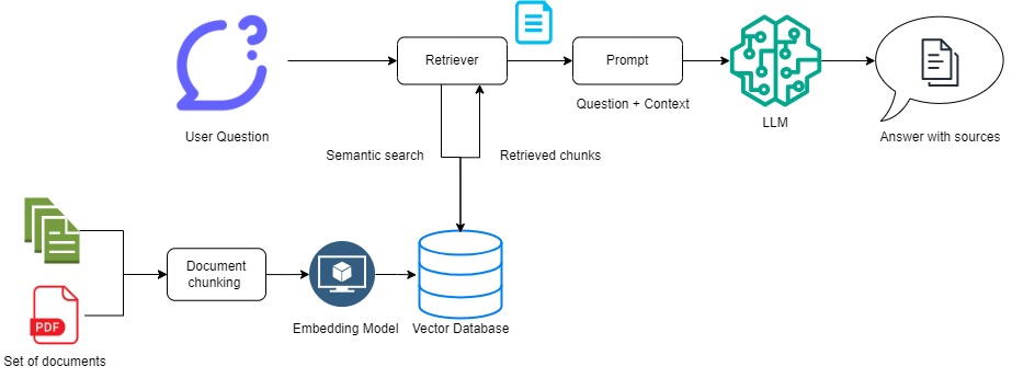
The diagram represents a simple RAG architecture.
Fig. 1 – RAG Architecture


The diagram above represents a simple RAG architecture. The system operates by initially directing the user’s question to a Retriever, which scans a vector database to locate relevant information chunks potentially containing the answer. Utilizing predefined metrics, it matches the embedded question with stored embeddings through similarity matching. Subsequently, identified relevant chunks are merged with the original question to construct a Prompt. These retrieved chunks serve as the context for the LLM to generate the answer. Finally, the system delivers the response to the user, often referencing the sources or documents from which the information was retrieved. In the process of ingesting documents, they are parsed only once, chunked with the appropriate chunking method, and stored in the vector database as vector embeddings for further querying. This ensures that documents are not ingested repeatedly, but rather stored efficiently for quick retrieval. These documents can originate from diverse sources such as PDF files, plain text files, markdown, Confluence, URLs, etc.


LlamaIndex’s VectorStoreIndex


During the construction of a straightforward RAG architecture with a limited number of documents, the VectorStoreIndex comes into play. But what exactly is the VectorStoreIndex? According to the creators of the LlamaIndex library, it is one of the most prevalent forms of an Index, which is a data structure created from objects of the Document type to facilitate inquiries by the LLM. The utilization of VectorStoreIndex can be approached in two ways: high-level or low-level. Each has its advantages and drawbacks. But first, let us discuss what they entail.


High level approach


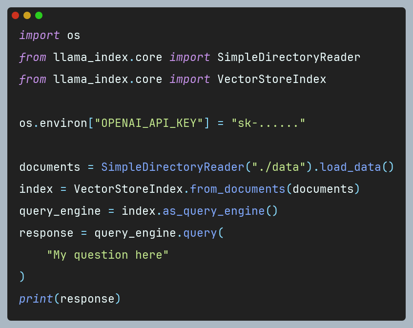
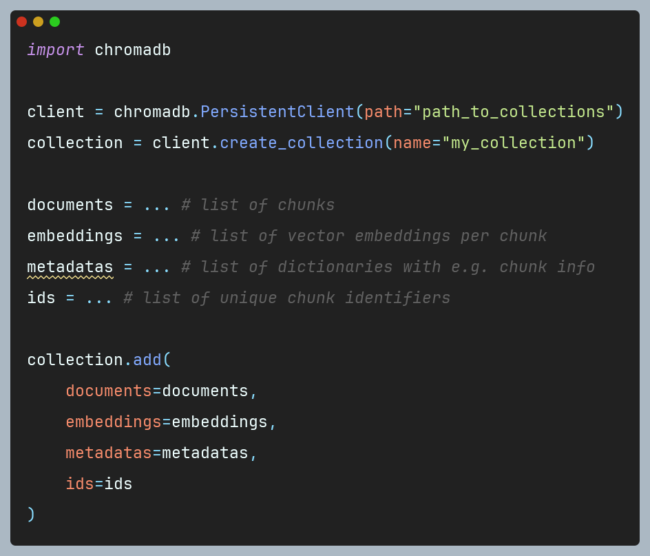
For each RAG architecture, documents must be loaded, parsed, and chunked in a certain way. If we have a small number of documents (for example: 5), we can use the SimpleDirectoryReader from LlamaIndex for this purpose. We can pass the full path to the folder containing all the files we want to read. It loads the documents from the given directory and returns them as a list of Document objects. Then, we provide them to the from_documents() method of VectorStoreIndex to create the Index – here our Documents are split into chunks and parsed to Node objects. In the final step, we call the as_query_engine() method on the Index, which creates the engine, and voila, we are able to query our documents. The described scenario is presented in the following code snippet:


High level approach scenario


Despite the ability to swiftly and with minimal effort pose queries to documents, the utilization of VectorStoreIndex in this scenario is not flawless. Here, we suffer from a lack of control over the underlying processes, as VectorStoreIndex autonomously chunks documents and computes embeddings. This lack of control may lead to less satisfactory results and may not always meet the user’s expectations. Responses can be less accurate or contain often irrelevant information with respect to the initial question, therefore, a more hands-on approach might be necessary to ensure higher quality outcomes.


Low level approach


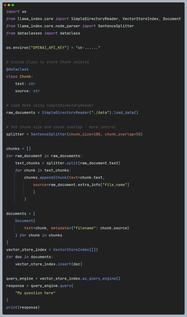
With a low-level approach, more effort is required, as we have the autonomy to directly decide how to load the data, parse it, and split it into chunks. Ready-made classes such as SentenceSplitter can be employed for this purpose, or one can implement their own chunking method, such as semantic chunking. Following this idea, we’ve implemented our own semantic chunking method called Semantic double-pass merging. We have described it in details and compared against another chunking methods in our article.


Assuming our data is loaded and transformed into chunks, we can utilize the insert() method of the VectorStoreIndex class to compute and store embeddings. However, it is essential to note that insert() requires a Document object as input, thus the chunks must be appropriately transformed. The following code snippet illustrates the described operation:


Low level approach scenario


This approach is significantly more flexible, providing greater control over what gets stored in the vector storage. Nonetheless, it should be noted that it entails a greater workload, with proper chunking being a crucial aspect. Low level approach fits great with popular statement “with great power comes great responsibility” meaning that the programmer holds the reins to ensure the quality of responses by selecting the proper chunking method, thresholds, chunk sizes and other parameters. While this approach offers potential for higher quality responses, it does not guarantee it with absolute certainty. Instead, it allows the developer to optimize and tailor the process to specific needs, making the outcome dependent on the developer’s knowledge and decisions.


In both cases, embeddings are computed underneath by LlamaIndex, inherently utilizing the OpenAI text-embedding-ada-002 model. By default, indexed data is kept in memory, as is the case with the above examples. Often, there is a desire to persist with this data to avoid the time and cost of re-indexing it. Here, LlamaIndex helps with the persist() method, further details of which can be gleaned from the LlamaIndex documentation. Alternatively, one can leverage an external open-source vector database such as Chroma.


Chroma – open-source vector database


In the case of a larger quantity of documents beyond just a few individual PDF files, keeping them in memory may not be efficient. Developing RAG system may consume significantly more documents over time, resulting in excessive memory allocation. In terms of scalability, external vector databases designed for storing, querying, and retrieving similar vectors come to the rescue. Most open-source databases are integrated with libraries like LlamaIndex or LangChain, offering even simpler utilization. In this section, we examine the Chroma database (in the form of chromadb Python library) with LlamaIndex.


Within chromadb framework collections serve as a repository for embeddings. This library presents a range of methods for proficiently managing collections, encompassing creation, insertion, deletion, and querying functionalities. The instantiation of a specific collection necessitates the involvement of clients. In scenarios where one seeks to persist and retrieve their collection from a local machine, the PersistentClient class comes into play. Here, data automatically persisted and loaded upon startup if it already exists.


The chromadb library offers flexibility in terms of embeddings creation. Users have the option to create collections and provide only the relevant chunks, whereby the library autonomously calculates the embeddings. Alternatively, users can compute their own vectors embeddings using, for instance, a custom-trained embedding model, and then pass them to the collection. In the case of entrusting Chroma with the computation of embeddings, users can specify their chosen model through the embedding_function parameter during the collection creation process. Furthermore, users can provide their own custom function if they intend to calculate embeddings in a unique manner. If there is no embedding_function provided, Chroma will use all-MiniLM-L6-v2 model from SentenceTransformers as a default. For further insights, detailed information can be found in the chromadb documentation.


In our example, we will focus on embeddings previously computed using a different model. It is crucial that regardless of the method employed for generating embeddings (whether through Chroma or otherwise), they are created from appropriately chunked text. This practice significantly influences the quality of the resulting RAG system and its ability to answer questions effectively. The following code snippet demonstrates the creation of a collection and addition of documents with embedding vectors:


creation of a collection and addition ofdocuments with embedding vectors


Chroma offers flexible storage of information within collections, accommodating both documents and their corresponding embeddings or standalone embeddings. Furthermore, by adding data to the collection using the add() method, one can specify a list of dictionaries in the metadatas argument, each corresponding to a particular chunk. This approach facilitates easy querying of the collection by referencing these metadata (further details on querying collections can be found in the documentation). This capability is particularly valuable for businesses needing to instantly search and retrieve the latest company-specific documents, thereby accelerating the process of finding nuances in documentation. As a result, it significantly enhances efficiency and decision-making, ensuring that critical information is readily accessible.


It is crucial to provide a list of document identifiers in the ids argument, as each document (chunk) must possess a unique ID. Attempting to add a document with the same ID will result in the preservation of the existing document in the collection (there is no overwrite functionality).


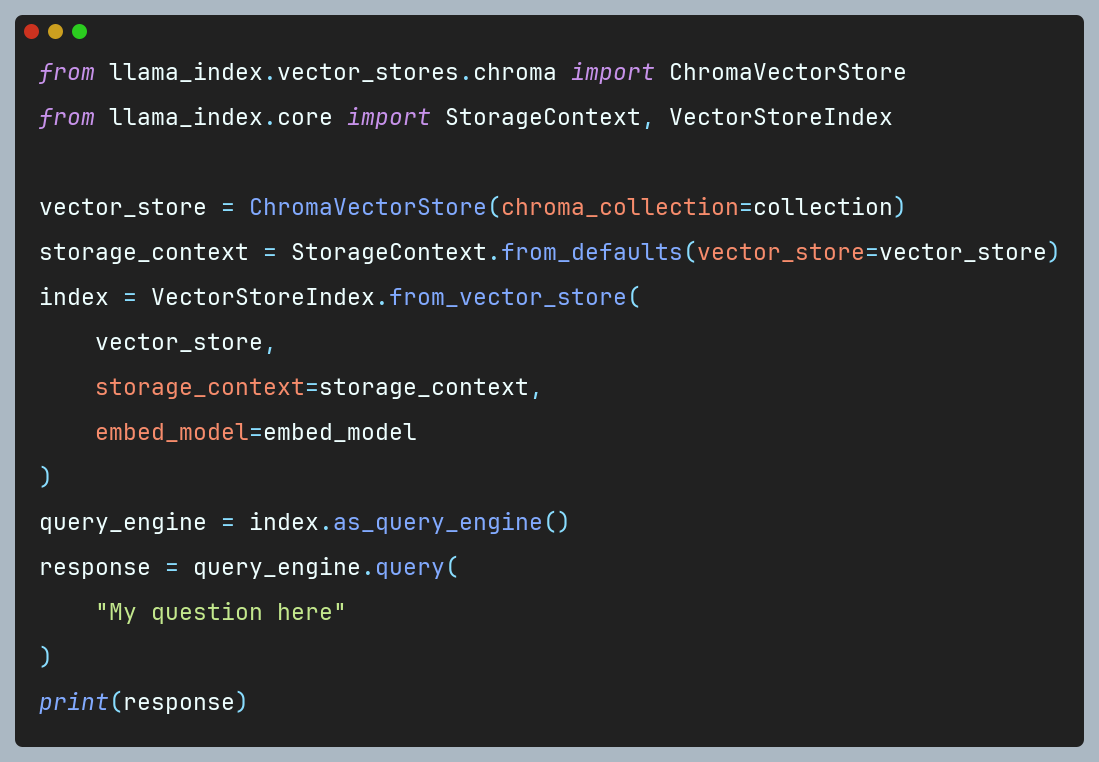
Once the collection with our embeddings is created, how can we use it with LlamaIndex? Let’s examine below code snippet:


Once the collection with our embeddings is created, how can we use it with LlamaIndex


Utilizing a previously established collection, we construct an instance of the ChromaVectorStore class. Subsequently, it is imperative to instantiate a StorageContext object, serving as a toolkit container for storing nodes, indices, and vectors – a crucial component utilized in the subsequent step to create an Index. In the final phase, an Index is formed based on the vector storage and its context. Here ChromaVectorStore object is transformed to VectorStoreIndex using the from_vector_store() method, effectively making the ChromaVectorStore represent the same object type as VectorStoreIndex. Here, it is also crucial to specify the embed_model parameter with the same embedding model that was used to compute embeddings from chunks. Providing a different model or omitting it will result in dimensional errors during querying. Following the creation of the Index, analogous to the VectorStoreIndex class, we establish an engine to field inquiries regarding our documents.


Embedding search methods


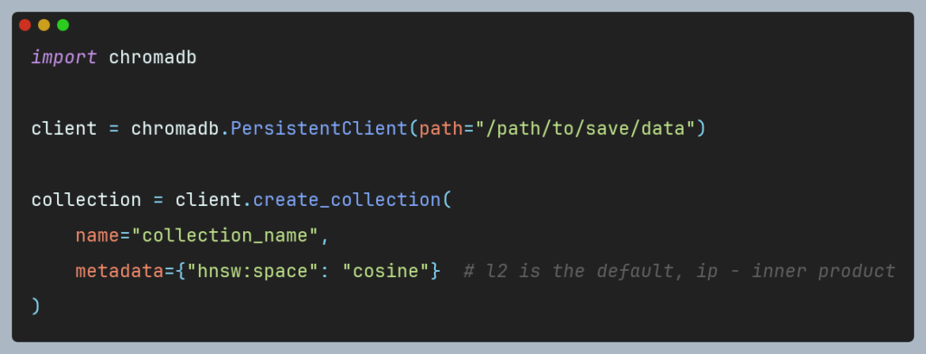
In previous technical sections, we discussed how to index custom documents to query them using natural language through two libraries: the built-in tools offered by LlamaIndex and the integration of Chroma with LlamaIndex. However, it is worth mentioning how these frameworks search for similar embedding vectors. In a vector space, to compare two vectors, one must perform a comparison operation using a mathematical transformation (metric similarity). The most used metric is cosine similarity, which is the default metric used by LlamaIndex. Conversely, Chroma defaults to the Squared L2 metric but also provides cosine-similarity and inner product, allowing users to choose the most suitable metric. Unfortunately, at the time of writing this article, it is not possible to change the cosine similarity metric in LlamaIndex, as it is hardcoded. In contrast, Chroma allows for metric selection easily by specifying it in the metadata parameter when creating a collection:


Chroma allows for metric selection easily by specifying it in the metadataparameter when creating a collection


Each similarity metric has its advantages and disadvantages, and the selection of a specific one should be made based on the developer’s best judgment. Cosine similarity, while the most popular and commonly used with vector embeddings, has its limitations, and should be used cautiously. For a deeper understanding of the nuances and potential pitfalls of using this metric, please refer to a detailed discussion in this article.


Summary


LlamaIndex with VectorStoreIndex and external vector databases like Chroma are fundamental tools for creating Retrieval-Augmented Generation systems. Both frameworks have been implemented and evaluated in our internal project to ingest and store vector embeddings from various data sources.


Regarding costs, LlamaIndex requires an OpenAI API key to calculate vector embeddings, as it uses the OpenAI text-embedding-ada-002 model by default, which incurs charges for each calculation. In contrast, Chroma employs open source embedding models, eliminating this cost.


For simpler RAG systems, involving a limited number of documents, VectorStoreIndex is a robust and effective choice. However, in real-world applications, the number of documents can grow rapidly, making in-memory storage inefficient. The natural solution is to use an external vector database to store this data. Several tools on the market facilitate integration with such databases, including LlamaIndex, which continues to evolve and offer new functionalities for efficient RAG construction.


It is important to note that storing documents and vector embeddings is just part of the equation. Equally crucial are the methods for parsing documents, appropriate chunking, and capturing the nearest chunks. These elements play a significant role in the overall performance and efficiency of RAG systems.


All content in this blog is created exclusively by technical experts specializing in Data ConsultingData InsightData Engineering, and Data Science. Our aim is purely educational, providing valuable insights without marketing intent.

bg

VectorStoreIndex vs Chroma Integration for LlamaIndex's vector embeddings - comparison

Dive deep into comparison of LlamaIndex’s VectorStoreIndex and LlamaIndex with Chroma integration for storing and querying vector embeddings with our Data Science Team.

Read more arrow

To effectively manage data, comply with legal regulations, and improve data-related business processes in every company, including the pharmaceutical industry, it is necessary to introduce data modeling standards. These standards bring the rules for storing, organizing, and accessing data, which is becoming increasingly important in the face of growing data complexity and regulatory requirements. The result is a solid data model that serves as a blueprint for designing and managing data structures. It ensures data consistency, reliability, and ease of access.


Importance of data modeling standards


Implementing data modeling standards is important for several reasons. Firstly, data should consistently ensure uniformity across various systems, databases, and departments, facilitating seamless data integration and communication​.


Pharmaceutical data, like any other, can have invalid values, differing measurement units, or missing attributes necessary for proper processing. Therefore, data teams responsible for data quality should understand these limitations before deciding on the conditions for using or not using the data. This is where it helps to have modeling standards that ensure standardization and high quality of data, manifested in increased accuracy, uniformity, and reliability.


From a business perspective, this is vital for faster decision-making and regulatory compliance​. For instance, promoting drugs to doctors and hospitals in the USA requires adherence to the Sunshine Act, mandating the reporting of payments made to individuals or institutions.


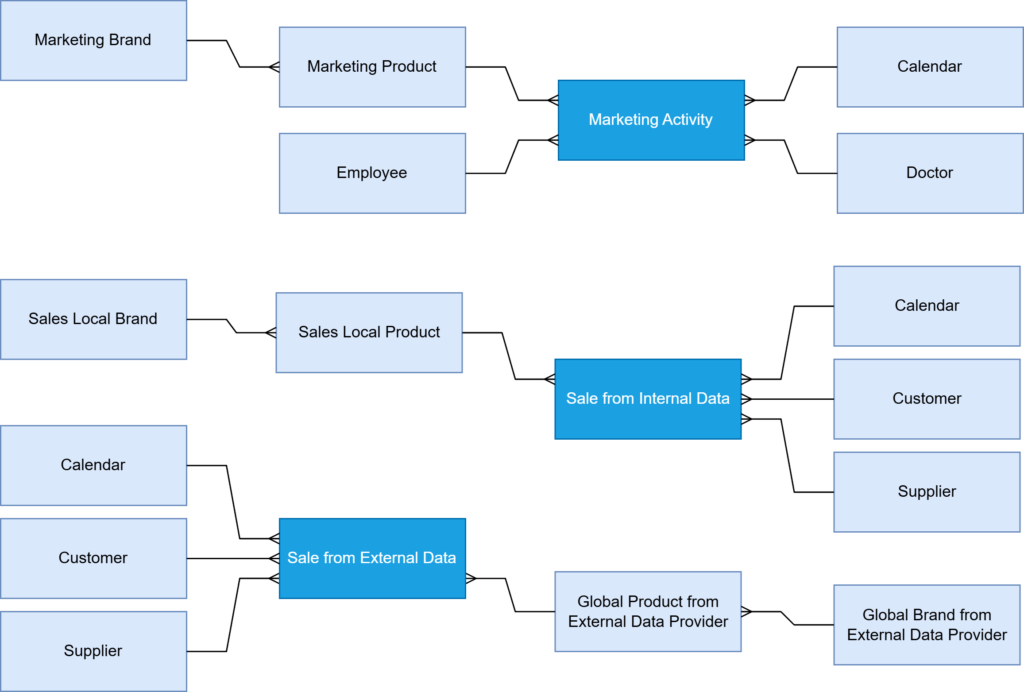
Another challenge is a large volume of data received, which must be collected, exchanged, and processed to provide holistic insights into business operations. A single standardized data model (example in Figure 1B) supports this by reducing data redundancy, as fewer data records need to be loaded into the data warehouse.


Additionally, data modeling standards facilitate collaboration across different departments of the enterprise by using the same data naming convention and following approved procedures. A shared understanding of the data model enables collaborative and informed business decisions based on consistent and accurate data while engaging a broader audience.


Example of a non-standardized data model in pharma
Figure 1A: Example of a non-standardized data model (before harmonizing brand and product data) in a pharmaceutical company, including the source-dependent brand and product dimensions.Example of a non-standardized data model (before harmonizing brand and product data) in a pharmaceutical company, including the source-dependent brand and product dimensions.


Example of a standardized data model in pharma
Figure 1B Example of a standardized data model (after harmonizing brand and product data) in a pharmaceutical company, including the unified brand and product dimensions.


Identification of key challenges in pharmaceutical data modeling


Pharmaceutical companies frequently encounter multiple challenges in implementing effective data modeling standards. These challenges start with the data itself, its quantity and complex structure, then their combination into one consistent data set, all while being limited by available resources and legal regulations.


One significant issue is the complexity of managing and integrating vast and diverse data sets from numerous sources and by different development teams. Reaching a consensus on objects that contain the same domain data stored across multiple systems, especially product data, is frequently difficult. Poor information governance around master data exacerbates organizational complexity, and a high degree of overlap in master data, such as customer data stored across various objects in the enterprise data model, is common.


Development carried out by independent teams, both internal and vendors’, forces coordination between them while expanding and optimizing the structure and content of the enterprise data warehouse. They must share the common knowledge of the data model, data modeling standards, and architectural principles. Changes introduced by them should be in accordance with approved procedures and documented in the same location and format.


Organizations often face significant challenges with data quality issues. These include master data such as customer and product information, as well as data from legacy systems with varying standards. The absence of a comprehensive MDM (Master Data Management) that defines different levels of data sources (primary and secondary) makes integration and expansion of the data model more difficult.


We encountered such challenges with one of our clients. To effectively address them, we assembled a team that included data management experts and consultants to help design and implement a robust data model and standards across the entire pharmaceutical company. In the next chapter, we describe how we coped with these challenges and why an appropriate approach to the data model strongly affects the quality and availability of business analytics.


Harmonizing brand and product data in a pharmaceutical company


A pharmaceutical company, one of BitPeak’s clients, needed to optimize an MDM system specifically for brand and product names by consolidating objects containing the same domain data from various sources. This initiative aimed to create a unified brand and product data hierarchy, standardize naming conventions, and integrate data from multiple database systems.


After preliminary workshops and a thorough pre-analysis conducted by BitPeak’s Business-System Analysts, the project focused on several key areas: data harmonization, content consolidation, updating and optimizing the MDM, and incorporating process automation wherever feasible to tailor the solution to client.


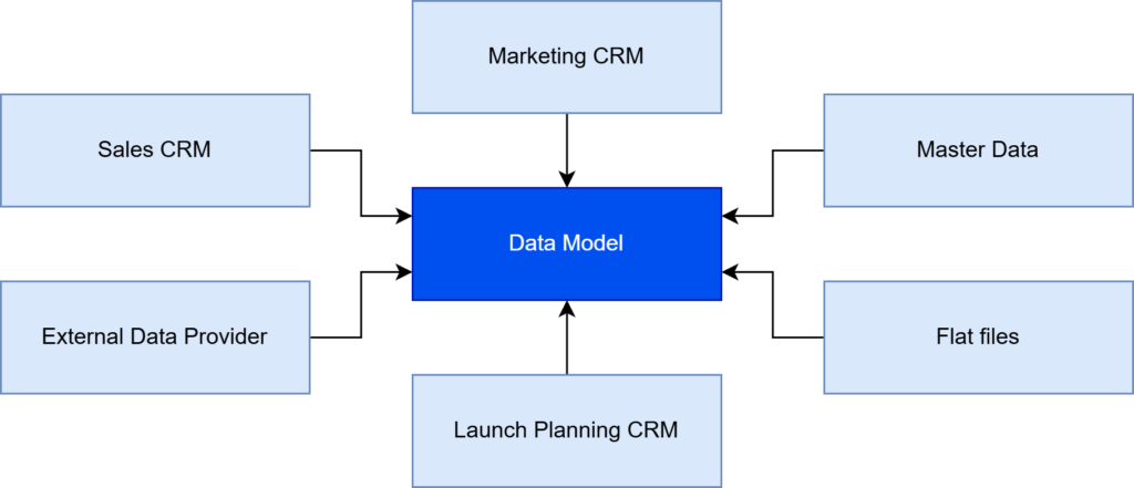
The process began with identifying the data sources that should be covered by the MDM. The client’s enterprise operates on a data model based on several different types of data sources (Figure 2):

  1. Sales CRM — containing both actual and historical sales transactions at a product level, offering a comprehensive view of sales performance.
  2. Marketing CRM — with data covering aspects of the employee’s marketing activities, including promotional efforts, campaigns, and customer engagement.
  3. Master Data — providing business objects that hold the most critical and universally accepted information, i.e. data dictionaries and hierarchies, shared across the organization, serving as the single source of truth.
  4. Flat files — with additional information required by the business, often used for ad-hoc reporting, or supplementary data that is not available in structured databases.
  5. Launch Planning CRM — for collecting data on the process before introducing products to the market, including timelines, projected quantities, and anticipated sales.
  6. External Data Provider — with sales data gathered by the global pharmaceutical data company, providing external benchmarks and insights to validate internally collected data.


General types of product-related data sources in pharma
Figure 2 General types of product-related data sources in a pharmaceutical company.


Data objects and specific fields requiring standardization were then selected. In our case, we focused on brand and product naming across the company’s diverse database systems. The client’s company departments were using incompatible global and local names (Figure 1A), making it much more difficult for data analysts to link information from various business areas (e.g., sales, marketing) and, consequently, track products at different stages of their life cycle in the market. Due to existing data inconsistencies, analyzing the data was challenging.


Designing the data model was the next crucial step. The Business-System Analyst, in collaboration with a Data Architect, developed a structured hierarchy for brand and product names (Figure 1B). This involved creating unified definitions and naming standards to ensure consistency across all platforms and compliance. The Development Team then prepared the environment for integrating data from various systems, migrating this data into a central master data repository.


Update of Master Data Management (MDM) system in a pharmaceutical company
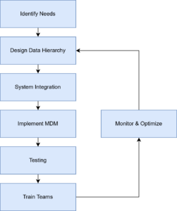
Figure 3 Update of Master Data Management (MDM) system in a pharmaceutical company.


Implementing changes in the MDM system required careful configuration according to the developed data hierarchy. The Development Team conducted rigorous integration and data consistency tests to ensure that the system functioned correctly, and that data integrity was maintained. Following successful integration, training sessions were organized for the marketing and sales teams, demonstrating how to use the MDM system and highlighting the benefits of having a unified database. Monitoring and optimization are continuous processes. Support kept track of the MDM system’s performance and collected feedback from users. They are then forwarded to an analyst for in-depth analysis and collection of business requirements. Any necessary adjustments and optimizations were implemented by the Development Team to enhance the system efficiency and user experience.


The project successfully delivered a unified data hierarchy for brand and product names. By gathering data in one consistent repository, it became more accessible and reliable, significantly improving the consistency and quality of marketing and sales analyses. Moreover, thanks to standardized brand and product names around the world, business awareness and knowledge about market performance on a global and local scale have increased. The reports obtained on their basis enable cross-interpretation of harmonized data sets from various data systems and getting a holistic image of the pharmaceutical company’s operations from the pre-launch process, through product implementation, marketing, to performance monitoring. This leads to making the right and more conscious decisions regarding the international pharmaceutical business.


Summary


At BitPeak, we always prioritize proactive cooperation with our clients, guided by the highest business value of the proposed data solutions. Therefore, we pay attention to effective data management and compliance with data modeling standards, which constitute the foundation for the good operation of any global company. By using recognized best practices and modern technologies, companies can increase the accuracy, consistency, accessibility, and regulatory compliance of their data. The result is better business intelligence that enables clients to make more informed decisions, contributing to gaining a competitive edge on the market.


All content in this blog is created exclusively by technical experts specializing in Data ConsultingData InsightData Engineering, and Data Science. Our aim is purely educational, providing valuable insights without marketing intent.

bg

Data model for pharma: key challenges and best practices

Discover the importance of implementing data modeling standards in the pharmaceutical industry to ensure compliance, enhance processes, and optimize data management.

Read more arrow

Introduction


This is the second article in our series about Environmental, Social, and Governance (ESG), a topic which is becoming increasingly more and more important both legally and economically. In part one of the series, we described what ESG is, why it is important, and what are current regulations. We highly recommend the read!


This time we would like to dive deeper into reporting aspects of ESG and explain why we think Microsoft Power BI together with Fabric ecosystem are the best options to both fulfil all the requirements and gain additional value and advantage over the competition. We will show an example of GRI standards compliant Power BI report and describe design choices, benefits of such a solution, and also possible enhancements like AI talking with data behind the report.


Business Intelligence…


Business Intelligence (BI) can be defined as a set of practices and tools allowing businesses to manage their data and analyze it for the benefit of the whole organization. Introducing BI can generate value in various ways like automating labor-intensive data-related tasks, standardizing reporting processes, granting observability for core company’s operations, enhancing decision making, and many more. Together with data governance, BI can bring order to your data assets and allow you to discover and focus on what are foundational metrics that drive your business.


Power BI allows organizations to easily connect to data from various sources, transform it, build data models, and create all possible metrics. This metrics layer built on top of a data model is known as a semantic layer – here business logic is superimposed on the data. Recent research papers (link) show that the semantic layer might be a crucial factor for AI to deliver precise answers and minimize hallucinations. Models built in Power BI can be scaled to enterprise level, and all the metrics can be presented on reports, furtherly enriching the whole solution by using best data visualization practices. As part of Microsoft Fabric (AI-powered analytics platform) and seamless integration with Power Platform (business applications), Power BI can fulfill almost any business need.


With addition of MS Fabric, Power BI is now part of a data platform based on modern Lakehouse architecture, with an integrated storage layer called OneLake and multiple workflows including data engineering, data science, and real-time intelligence. With such a setup Power BI can consume best quality, well-governed data from almost any source. It is also worth noting that any part of this platform will be integrated with AI, able to handle most of the repetitive tasks, significantly increasing productivity.


Power Platform is a mature solution where less technical users can create business applications (Power Apps), automations (Power Automate), and AI agents (Power Virtual Agents) on top of organizational data, which can reside almost anywhere thanks to the great number of connectors. It can also reside in MS Fabrics and Power BI. This creates a situation where users can enrich organizational data in multiple ways and significantly simplify processes like approvals, alerts, surveys etc.


Before we go further, let us make sure we are all on the same page, by answering the basic question. What exactly does ESG mean?


…with ESG…


Let’s try to look at ESG reporting from a Business Intelligence perspective. It might be a challenge for many organizations to effectively create an ESG report as various data sources need to be evaluated and data needs to be collected. Depending on the size of the organization the level of complexity here may vary, from manual collection of necessary numbers in Excel, to a fully sized ETL/ELT pipeline. Data might be located outside of the organization (e.g., water or energy suppliers or companies that collect waste) or inside (financial or HR departments).


Typically, this data collection phase might be the biggest challenge, but it can be simplified with automation of data ingestion  data from some sources can be ingested directly by Power BI (e.g., with CSV/Excel files or via API), through Power Apps, or by using data engineering pipelines. With data in place, a work on fully automated, interactive reporting solution can start.


Recently at BitPeak, we created a GRI-compliant ESG report (link) and we will use it as an example. GRI stands for Global Reporting Initiative –  an organization that creates standards that can serve as a framework to report on business impacts, including the ones in the scope of ESG (link).


It is worth noting that GRI standards are international and widely adopted across companies (78% of 250 biggest global companies adopted those standards). European Union used GRI standards and other frameworks to create ESRS European Sustainability Reporting Standards, which are used by large companies in the EU to report on their ESG goals. ESRS can be easily mapped to GRI standards which is visible in the matrix further below.


There are several categories covered by GRI standards and for each one of them, there is a set of metrics that describe it in the best possible way. In our report, we show the following categories:

  • GRI 200: Economic Reporting
  • GRI 300: Environmental Reporting
  • GRI 400: Social Reporting


In each category, we may find both descriptive and quantitative KPIs and for our solution, we decided to choose the latter ones – for those, their progress can be easily tracked. Some examples can be found below (ESRS mapping included):


Area Indicator GRI Code ESRS code
ENVIRONMENT ENERGY CONSUMPTION 302-1 ESRS E1 E1-5 §37; §38; §AR 32 (a), (c), (e) and (f) (some differences in how data is aggregated/disaggregated)
ENVIRONMENT WATER USAGE AND WITHDRAWALS 303-5 ESRS E3 E3-4 §28 (a), (b), (d) and (e)
ENVIRONMENT GREENHOUSE GAS EMISSIONS 305-1 ESRS E1 E1-4 §34 (c); E1-6 §44 (a); §46; §50; §AR 25 (b) and (c); §AR 39 (a) to (d); §AR 40; AR §43 (c) to (d)
ENVIRONMENT GREENHOUSE GAS EMISSIONS 305-2 ESRS E1 E1-4 §34 (c); E1-6 §44 (b); §46; §49; §50; §AR 25 (b) and (c); §AR 39 (a) to (d); §AR 40; §AR 45 (a), (c), (d), and (f)
ENVIRONMENT GREENHOUSE GAS EMISSIONS 305-3 ESRS E1 E1-4 §34 (c); E1-6 §44 (c); §51; §AR 25 (b) and (c); §AR 39 (a) to (d); §AR 46 (a) (i) to (k)
ENVIRONMENT EMISSIONS OF AIR POLLUTANTS 305-4 ESRS E1 E1-6 §53; §54; §AR 39 (c); §AR 53 (a)
ENVIRONMENT WASTE GENERATION AND DISPOSAL 306-3 ESRS E5 E5-5 §37 (a), §38 to §40
ETHICS RISK CORRUPTION ANALYSIS 205-1 ESRS G1 G1-3 §AR 5
ETHICS REPORTED CASES OF CORRUPTION 205-3 ESRS G1 G1-4 §25
ETHICS LEGAL ACTIONS TAKEN 206-1 Not covered
ETHICS CUSTOMER PRIVACY BREACHES 418-1 ESRS S4 S4-3 §AR 23; S4-4 §35
LABOR & HUMAN RIGHTS EMPLOYEE TURNOVER RATE 401-1 ESRS S1 S1-6 §50 (c)
LABOR & HUMAN RIGHTS OCCUPATIONAL HEALTH AND SAFETY INCIDENTS 403-9 ESRS S1 S1-4, §38 (a); S1-14 §88 (b) and (c); §AR 82
LABOR & HUMAN RIGHTS TRAINING AND DEVELOPMENT HOURS 404-1 ESRS S1 S1-13 §83 (b) and §84
LABOR & HUMAN RIGHTS DIVERSITY IN THE WORKFORCE 405-1 ESRS 2 GOV-1 §21 (d); ESRS S1 S1-6 §50 (a); S1-9 §66 (a) to (b); S1-12 §79
LABOR & HUMAN RIGHTS NON-DISCRIMINATION INCIDENTS 406-1 ESRS S1 S1-17 §97, §103 (a), §AR 103
SUPPLY CHAIN PERCENTAGE OF LOCAL SUPPLIERS 204-1 Coveredy by MDR-P, MDR-A, MDR-T
SUPPLY CHAIN SUPPLIER ASSESSMENTS FOR SOCIAL AND ENVIRONMENTAL PRACTICES 414-1 ESRS G1 G1-2 §15 (b)


… and Power BI!


It is worth noting that creating a report with specific branding in mind is always welcome. With Power BI it is possible to add company logo, photos, or animations to report pages and apply required colors or patterns to multiple objects and charts.  For our report, we aligned with color guidelines applicable to our company. We also tried to mimic the website design by using specific shapes and fonts, so the report looks coherent and can be immediately associated with our brand.


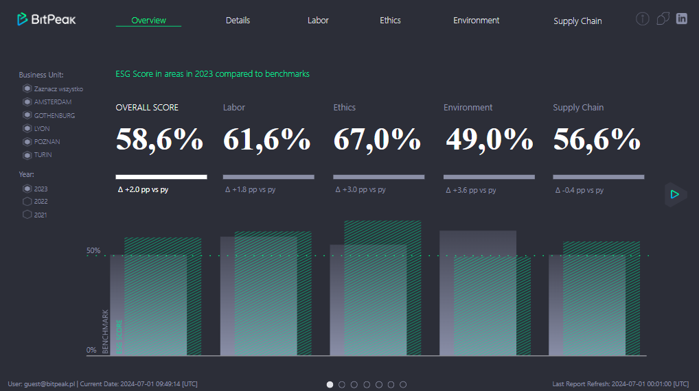
A dashboard from BitPeak in Power BI displaying the ESG (Environmental, Social, and Governance) score.


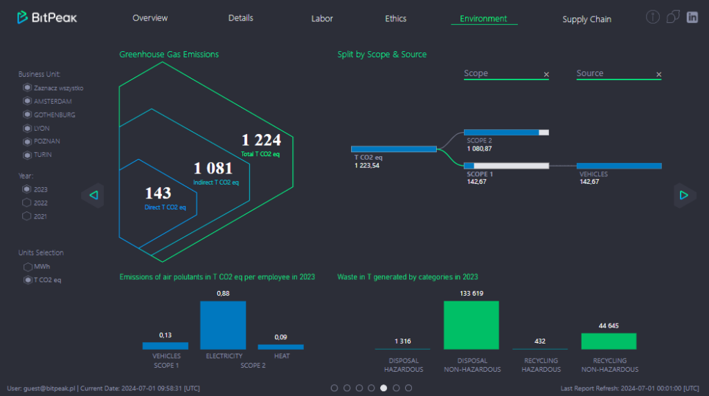
As visible above, the report has a clean design and an easy-to-follow structure. At the top we can see the company’s logo and navigation menu starting with the “Overview” page. As it is the first page that users see, we followed the helicopter’s view approach, where most top-level metrics can be analyzed with a glance of an eye. A user can then filter this page using the slicers on the left. In case a more granular access is needed, row-level security can also be applied – some users would see everything while others only slice of the data. We decided to use scores as a top-level KPIs – they could be either calculated using the company’s internal logic or by external auditors. In case the audience needs more detailed information, they can move on to either the details page, being a granular view, or to the specific domain page to find answers.


A screenshot of the Details tab within BitPeak Power BI, showcasing various data metrics and visual elements that provide in-depth insights into specific datasets,.


On “Details” page we present a matrix with a list of KPIs that correspond to score values. Targets set up by the leadership are also added, so that it is evident to users that some metrics needs to be furtherly evaluated. Area charts showing changes of scores in time, can help to distinguish if situation is improving or not. Depending on requirements the matrix can be modified to show the difference between the current and previous year, a drill-through option can also be added to make this page even more useful.


 A screenshot of the Environment tab in BitPeak Power BI, displaying various data metrics and visual elements that offer in-depth insights into specific datasets, including graphs, charts, and performance indicators for environmental data analysis.


Pages “Labor”, “Ethics”, “Environment”, and “Supply Chain” dive deeper into each category’s nuances. Again, we apply our company’s branding elements to create a familiar experience for our business users. It is important to remember that the report’s audience can consist of users that are not really fluent in reading charts and graphs, so on each page we try to use simple, but the most effective data visualizations, so that all the metrics can be easily interpreted. The decomposition tree is a fine example of a simple visual that can bring a lot of value to users, due to the fact that it allows them to easily explore data in various ways.


Potential improvements


Typically, BI projects are not static or one-time efforts. Usually after the evaluation period some adjustments are required, new functionalities are needed, and the whole solution grows. Therefore, let’s try to imagine how to leverage available technical options to enrich our report:


Breaking data silos


It is always worth looking at the reporting solution as a part of a bigger analytics architecture. ESG reporting can be integrated with finance, HR, or production reporting so that we can break data silos and see the whole picture. Insights coming from the ESG report can improve multiple business areas such as sustainability, employee wellbeing, or risk management. With all the company’s departments having a clear view of ESG goals, joint effort to reduce some of the impacts can be taken.


Action on data:


Power Platform


Addition of Power Apps and Power Automate can turn our modest report into robust business solution. Data validation can be easily added to the report’s canvas along with comments and data write-back. Certain actions can be triggered from the report itself including approvals, sending notifications, even implementing complex logic with Azure Functions or Logic Apps.


Data Activator (Fabric only)


If our data is stored in Microsoft Fabric then we have several new options to use. The first one to mention is Data Activator – a brand new workflow to monitor data and create alerts. It allows automation of the metric checks with highly customizable settings. Users can apply specific rules to alerts and can choose different ways to being notified (e.g., via email or Teams). What is important, is a low-code option so no coding skills are needed to use it.


Microsoft Copilot (Fabric only)


A very hot topic at the moment is using AI on your data. What Microsoft proposes is Copilot, an umbrella term to describe several AI agents that help users with tedious tasks. At the moment Copilot is available in multiple Fabric workflows. But for us, the most exciting one is the one that can work with Power BI’s semantic model and answer business questions. Earlier Q&A visual could do a similar thing but with the introduction of LLMs, it is a leap forward to deliver a more sophisticated solution.


Diamond Layer (Fabric only)


In Fabric, it is possible to connect to Power BI’s semantic model with a newly-created Python library called SemPy. Data stored in semantic models is especially valuable as it is clean, curated, and business logic is already incorporated here. That’s why it is sometimes called a “diamond layer” in medallion architecture. The option to connect directly to the model is called a Semantic Link and it opens tons of possibilities for users with coding skills. Data science workflows, data validation and QA or even model development can be done using this library.


Summary


The marriage of ESG and business intelligence can bring a lot of value to organizations. Reporting solution which grants observability and delivers actionable insights is the most visible outcome, but several equally important processes like evaluation of useful data sources, building scalable data pipelines, bringing data governance and establishing proper data culture take place allowing the company to grow and flourish.


If you would like to know more about how BitPeak can leverage your data estate to deliver enterprise-scale ESG solutions do not hesitate to contact Emil Janik, Head of Data Insights at BitPeak.


All content in this blog is created exclusively by technical experts specializing in Data ConsultingData InsightData Engineering, and Data Science. Our aim is purely educational, providing valuable insights without marketing intent.

bg

Data&ESG - part 2: Power BI dashboard

Take a Peak and learn a Bit about creating effective and easy-to-use Power BI dashboard for your ESG reporting needs!

Read more arrow

Introduction


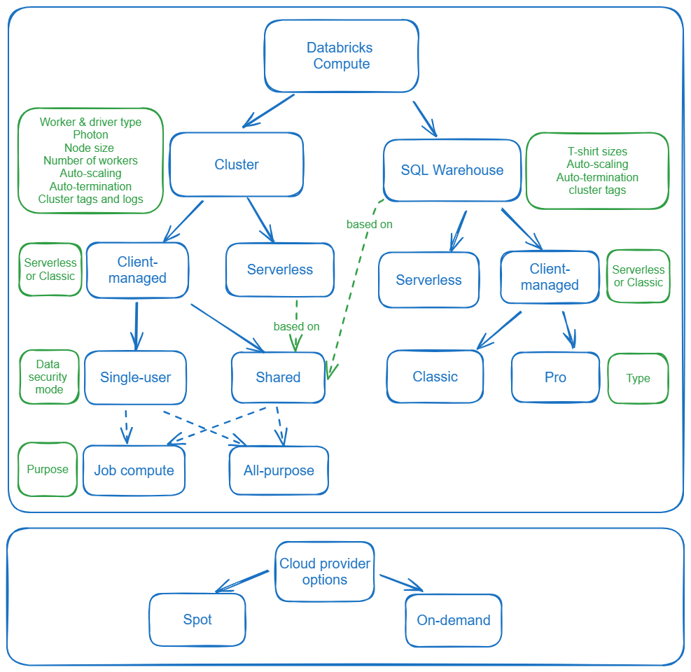
Databricks compute is a complex and deep topic, especially when considering the fact that the platform changes over time dynamically. Therefore, we would like to share a little know-how about choices that need to be made when deciding between compute approaches in specific use cases. Additionally, we will look over some compute management options not omitting serverless.


So, take a Peak at an article below and learn a Bit with our Databricks Architect Champion.


A graph illustrating Databricks compute resources, showcasing different compute options.


Job and all-purpose clusters


The all-purpose clusters are designed for interactive/collaborative usage in development, ad-hoc analysis, and data exploration while job clusters run to execute a specific, automated job after which they immediately release resources.


In case you need to provide immediate availability of a job cluster (for example for jobs that run very frequently and you cannot afford the ca. 5-minute startup time) consider using cluster pools and having a number of idle instances greater than 0.


Spot instances


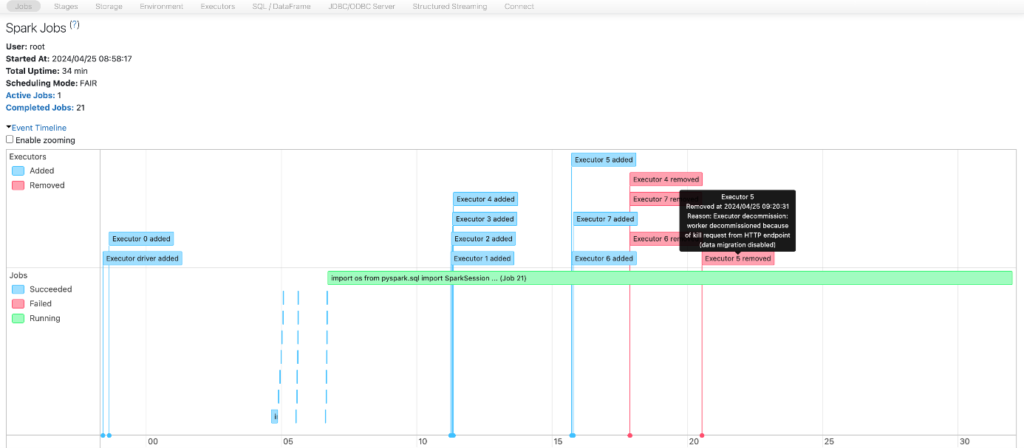
Spot instances (VMs) make use of the available compute capacity of a cloud provider with deep discounts. Databricks manages termination and startup of spot workers, so that the defined number of cores is reached and available for the cluster. Any time when cloud provider needs the capacity the machine is evicted, if you enable decommissioning – with an earlier notice. For Azure the notification is sent 30 seconds before the actual eviction (Use Azure Spot Virtual Machines – Azure Virtual Machines | Microsoft Learn).


spark.storage.decommission.enabled true
spark.storage.decommission.shuffleBlocks.enabled true
spark.storage.decommission.rddBlocks.enabled true


A screenshot of the Spark UI displaying information related to the decommissioning of a cluster node using spot instances,
Figure 1 Information in Spark UI when cluster node using spot instances is decommissioned


Using the above Spark configuration you can try to mitigate negative results of compute node eviction. The more data is migrated to the new node the less likely are the errors from shuffle fetching failures, shuffle data loss and RDD data loss. Even if a worker fails, Databricks manages its replacements and minimizes the impact on your workload. Of course, the driver is critical and should be kept as on-demand instance.


Databricks states decommissioning is a best effort so it’s better to choose on-demand instances for crucial production jobs with tight SLAs.


You can setup spot instances via Databricks UI but more options are available when using Databricks REST API (Create new cluster | Clusters API | REST API reference | Azure Databricks, azure_attibutes object), e.g., how many first nodes of the cluster (including driver) are on-demand, fallback option (you can choose to fall back to on-demand node), as well as the maximum spot price.


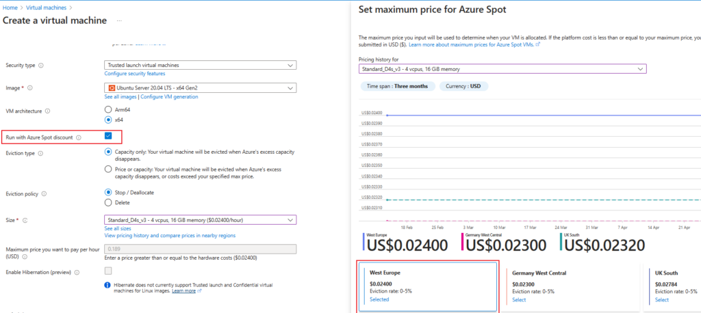
The spot price and a rough estimate of eviction rate for a region can also be checked in “Create a virtual machine” screen. For example, for West Europe region the eviction rate is 0-5%.


A screenshot showing the process of creating a virtual machine in Azure, with a highlighted option to set the maximum price for Azure Spot instances, illustrating the configuration settings for cost management during VM deploymen


It is important to note though, that storage and network IO are billed independently of the chosen option, at a regular price.


Single user or shared access mode


The single-user cluster is assigned to and can be used by only one user at a time while shared clusters are designed to be used by multiple users simultaneously thanks to the session and data isolation.


Both access modes work with Unity Catalog although the main limitation of the single-user cluster is that it cannot query tables created within UC-enabled DLT pipelines (also including materialized views created in Databricks SQL). To query such tables, you must use a shared compute.


There are still significantly more limitations on shared clusters due to the fact that these clusters need to provide session isolation between users and prevent them from accessing data without proper UC permissions (e.g., bypassing through DBUtils tools and accessing cloud storage directly):

  • You cannot manipulate with DBUtils, RDD API or Spark Context (instead you should use Spark Session instance).
  • Spark-submit jobs are not supported.
  • Language support: Scala supported on DBR 13.3 and above, no support for R.
  • Streaming limitations: unsupported options for Kafka sources and sinks, Avro data requires DBR 14.2 or above, new behavior for foreachBatch in DBR 14.0 and above.
  • No support for Databricks Runtime ML and Spark ML Library (MLib).


For comprehensive information on limitations consult Databricks documentation.


Databricks recommends using shared access mode for all workloads. The only exception to use the single-user access mode should be if your required functionality is not supported by shared access mode.


Cluster node type


When choosing node type for driver and worker you need to consider the performance factors which are most accurate for your specific job.

A cluster has the following factors determining performance:


  • Total executor cores: total number of cores across all workers; determines the maximum parallelism of a job.
  • Total executor memory: total amount of RAM across all workers; determines how much data can be stored in memory before spilling it to disk.
  • Executor local storage: the type and amount of local disk storage; Local disk is primarily used in the case of spills during shuffles and caching.


A good practice is to provide a separate cluster or cluster pools for different groups of interest. Depending on the workload to be run on a cluster you can configure memory and cores appropriately:


  • Ad-hoc analysis – Data analysts cluster’s main purpose is to pull, aggregate data, and report on it. SQL analysts use repetitive queries which often involve shuffle (wide) operations like joins or grouping. Therefore, both memory as well as local storage will be crucial factors. Consider using memory- or storage-optimized (with Delta caching) node types which will support repetitive queries to the same sources. There might be significant time gaps between running subsequent queries hence the cluster should have reasonable auto-termination minutes configured.
  • Training ML Models – Data scientists often need to cache full dataset to train the model. Hence, memory and caching are in high demand. In some cases, they might also need GPU-accelerated instance types to achieve highly parallelized computations. Therefore, the chosen compute type could either be storage-optimized or GPU-optimized compute.
  • For batch ETL pipelines the amount of memory and compute can be fine-tuned. Based on spark.sql.files.maxPartitionBytes setup (128 MB by default) as well as size of the underlying files we can estimate how many partitions will be created and assign an appropriate number of cores depending on parallelism and SLA we need to provide. If ETL jobs involve full file scans with no data reuse we should be good with compute-optimized instance types.
  • Streaming jobs usually have priority to compute and IO throughput over memory. Hence, compute-optimized instances might be a good choice. In case of streaming jobs of high importance, the cluster should be designed to provide fault tolerance in case of executor failures, so opt to choose more than one executor.


If workers are involved in heavy shuffles (due to wide transformations) you should also limit the number of executors, i.e., rather have more cores on one executor than having more executors with a small number of cores. Otherwise, you will put significant pressure on network IO which will slow down the job.


On the other hand, if an executor has a large amount of RAM configured this can lead to longer garbage collection times. Therefore, it should be tested when optimizing the size of the executor node whether you see any performance degradation after choosing a small number of workers.


When choosing a machine type you can also take a look at VM price comparisons on CloudPrice website (Azure, AWS, GCP Instance Comparison | CloudPrice) but remember that this is only what you pay to the cloud vendor for the VM. For example, even if a machine is shown here as a cheaper option you need to take into account also if it doesn’t incur higher DBUs costs as well as possibly a higher price for disk, if you change to an SSD-equipped machine.


Compute management


It is recommended to limit users’ ability to create their own fully-configurable clusters. Make sure you do not allow “Unrestricted cluster creation” to users or user groups unless they are privileged users. Instead, you can create several cluster policies addressing the needs of different groups of users (e.g., data engineers, SQL analysts, ML specialists) and grant CAN_USE permission to the respective groups.


You can control (i.e., hide or fix) multitude of cluster attributes. To name just a few:

  • Auto-termination minutes
  • Maximum number of workers
  • Maximum DBUs per hour
  • Node type for driver and worker
  • Attributes related to chosen availability type: on-demand or spot instances
  • Cluster log path
  • Cluster tags


With cluster policies each user can create their own cluster, if they have any cluster policy assigned, and each cluster has its separate limit for the compute capacity.


If there is a need to further restrict users, you can also limit users’ ability to create a cluster (assigning only CAN RESTART or CAN ATTACH TO permissions) and force users to only run their code on pre-created clusters.


Photon


In some cases Photon can significantly reduce job execution time leading to overall lower costs, especially considering data modification operations.


A valid case is when we would like to leverage dynamic file pruning in MERGE, UPDATE, and DELETE statements (which includes apply_changes in DLT world). Note that only SELECT statements can use this feature without Photon-enabled compute. This might improve performance, especially for non-partitioned tables.


Another performance feature conditioned by Photon is predictive IO for reads and writes (leveraging deletion vectors). Predictive IO employs deletion vectors to enhance data modification performance: instead of rewriting all records within a data file whenever a record is updated or deleted, deletion vectors are used to signal that certain records have been removed from the target data files. Supplemental data files are created to track updates.


Cluster tags and logs


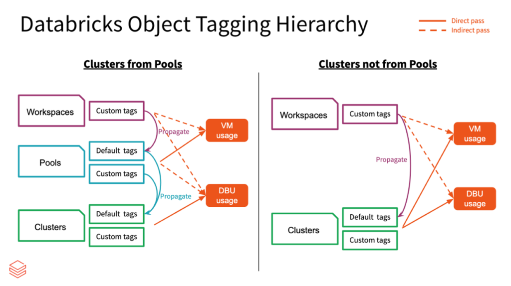
Last but not least, don’t forget to tag your clusters and cluster pools.


As you can see from the following graph tags from cluster pools will appear on associated cloud resources as well as are propagated to clusters created from that pool providing basis for DBU usage reporting. Hence, it is crucial, when using cluster pools, to pay attention to their tagging.


The tags are applied to cloud resources like VMs and disk volumes, as well as DBU usage reports.


A graph illustrating the Databricks object tagging hierarchy, displaying the relationship between different object types
Material from official Databricks documentation – Monitor usage using tags – Azure Databricks | Microsoft Learn


You might also consider specifying a location on DBFS (Databricks on AWS also support S3) to deliver the logs for the Spark driver node, worker nodes, and events, so that you can analyze the logs in case of failures or issues. The logs are stored for up to 30 days.


Serverless


As our article is meant to provide an overview of compute, we definitely cannot skip serverless which is becoming increasingly significant in Databricks environment.


Security


First concern when it comes to serverless is security.

Enterprises may have security issues with the compute running inside of Databricks cloud provider subscription (and not in customer’s virtual network).


Therefore it is important to take note of the available security features for serverless.

First of all, connection to storage goes always over cloud network backbone and not over public internet.


Secondly, you can enable Network connectivity configuration (NCC) on your Databricks account and assign it to your workspaces. You can choose either one of the two options to secure access to your storage accounts:

  • Using resource firewall: NCC enables Databricks-managed stable Azure service subnets which you can add to your resource firewalls
  • Using private endpoints: the private endpoint is added to an NCC in Databricks account and then the request needs to be accepted on the resource side.


Also, when considering serverless review the compute isolation and workload protection specification: Deploy Your Workloads Safely on Serverless Compute | Databricks


Serverless usage


Databricks serverless compute is definitely in expansion phase taking into consideration public preview features like serverless compute for workflows and notebooks as well as DLT serverless in private preview.


Here is a quick overview of the serverless compute features:

  • Fully managed compute,
  • Instant startup, usually ca. 5-10 seconds
  • Automated optimizing and scaling: selecting appropriate resources such as instance types, memory and processing engines,
  • Photon automatically enabled,
  • Automated retry of failed jobs (serverless compute for workflows),
  • Automated upgrades of Databricks Runtime version,
  • Based on shared compute security mode. Hence, all limitations of shared compute apply,
  • Serverless comes with pre-installed libraries (Serverless compute release notes – Azure Databricks | Microsoft Learn) but there is also an option to define your environment or install libraries in the notebook using pip,
  • Public preview of serverless compute does not support controlling egress traffic and therefore you cannot set up an egress IP (jobs have full access to the internet),
  • No cloud provider costs (only Databricks costs based on DBUs) but companies may not be able to leverage their existing cloud discount.


There is an obvious trade-off between having control over compute configuration and a fully-managed service that serverless is: you lose the ability to optimize the cluster and adjust instance types for your specific workload as well as you cannot choose the Databricks Runtime, which may result in compatibility issues.


Summary


As you can see, Databricks compute configuration presents pletora of options with which you can configure it to your needs. Each one has its advantages and disadvantages. Hopefully with this article you will be better equipped to wade through the settings and choose the best, most cost efficient option.


All content in this blog is created exclusively by technical experts specializing in Data ConsultingData InsightData Engineering, and Data Science. Our aim is purely educational, providing valuable insights without marketing intent.

bg

Databricks compute: overview and good practices

The newest Databricks compute method comparison by our Solution Architect Champion

Read more arrow

Introduction

In recent years Environmental, Social, and Governance (ESG) went from a secondary concern or bullet point on a CSR leaflet to a key part of corporate strategies. Why?

There are many reasons from research indicating that sustainability is good for a company’s long-term success to legal obligations, criteria for cheaper financing, and better employee relations. Aligning business and ESG strategies is both a challenge to overcome and an opportunity to seize.


Fortunately, both of which can be simplified thanks to advanced data gathering, analytics, and reporting tools, which allow companies to monitor their supply chains, forecast ESG risks, and keep up with new regulations. In our series of articles, we will guide you through the whole process


Understanding ESG


Before we go further, let us make sure we are all on the same page, by answering the basic question. What exactly does ESG mean?


E stands for the environmental criteria, which consider how a company performs when preserving and mitigating the harm to the natural environment. This can mean:

  • Renewable Energy Adoption: Companies investing in solar panels, wind turbines, or purchasing green energy to power their operations.
  • Waste Reduction Initiatives: Implement recycling programs, reduce packaging materials, and promote reusable products.
  • Sustainable Resource Use: Utilizing sustainable materials in production and adopting practices that reduce water consumption and prevent deforestation.
  • Carbon Footprint Management: Engaging in carbon offsetting projects and striving for carbon neutrality through various environmental initiatives.


S stands for the social criteria, which assess a company’s capacity and performance in managing relationships with communities around it, employees, shareholders, or, simply put – stakeholders. For example:

  • Fair Labor Practices: Ensuring fair wages, safe working conditions, and adhering to labor laws; promoting diversity and inclusion within the workforce.
  • Community Engagement: Investing in local communities through philanthropy, volunteer programs, and supporting local economic development.
  • Supply Chain Responsibility: Monitoring suppliers to ensure they adhere to ethical practices, including human rights and environmental standards.
  • Product Responsibility: Ensuring products are safe, meet quality standards, and are produced ethically, including respecting customer privacy and data protection.


G represents the Governance criteria, which revolve around the rules, practices, and processes by which a company is directed and controlled. Governance in the ESG context focuses on how a company ensures that its operations are transparent, compliant, and aligned with the interests of its shareholders and other stakeholders. This involves:

  • Board Structure and Composition: The effectiveness of the board in providing oversight, including its size, composition, diversity, and the independence of its members.
  • Ethics and Compliance: The company’s commitment to ethical behavior and compliance with laws, regulations, and internal policies, including mechanisms for preventing and addressing corruption and bribery.
  • Executive Compensation: How executive compensation is structured and aligned with the company’s long-term goals, performance, and shareholder interests.
  • Risk Management: The processes in place to identify, manage, and mitigate risks that could affect the company’s business, reputation, and long-term sustainability.
  • Shareholder Rights and Engagement: Ensuring that shareholders have a voice in important decisions through voting rights and other engagement mechanisms , and that their interests are considered in the company’s governance practices.


Why is ESG important?


Now we know what ESG is. But why should you care about it? Aside from ethical reasons.
The present relevance of ESG is underpinned by its integration into investment decisions, corporate strategies, and regulatory frameworks during the last few years.


For many bigger companies, those who are included in increasingly numerous sustainability regulations, ESG compliance is no longer optional, though for now, it is mostly focused on reporting and prevention of greenwashing, such as SFRD and CSDR. Even if they are  omitted, they probably want to work with those who are or obtain financing from ESG-focused funds. Especially since some of the biggest financial management funds, such as Blackrock, steer increasingly in the ESG direction.


However, the question of the permanence of such direction persists as recently some moved away from sustainability-focused funds.


Sustainability factors can influence investor preferences, government grants, consumer behavior, and financing possibilities. Because of that ESG-compliant financial assets are projected to exceed $50 trillion by 2025, accounting for more than a third of the projected $140.5 trillion in global assets under management. This significant growth, from $35 trillion in 2020, reflects the increasing mainstreaming of ESG criteria into the financial sector and beyond​​​​.


The research also indicates that ESG funds outperform their less sustainable counterparts over both shorter and longer periods of time.


It is also worth noting that there is no “Too big for ESG”. Tech giants such as Amazon, Google, and Apple, have faced scrutiny regarding their ESG practices, especially in the social and governance aspects. This not only made them eat bad PR but also motivated regulators to take a closer look at them.


This means that the growth of ESG assets and the increasing integration of ESG criteria into business practices reflect a paradigm shift in the business and investment landscape. And as sustainable governance becomes more critical, companies are urged to adopt comprehensive strategies to meet new, evolving standards, and ensure that their operations align. Well, and report everything about that alphabet soups such as CSRD, or SFDR or CSDDD requires them to.


Knowing all that, let us ask about what new challenges will appear and how to make ESG strategy an asset rather than bothersome new obligations. We will start by identifying business and legal challenges and risks.


Business & legal – challenges and opportunities


First, let’s take on business challenges, which consist mostly of strategic and operational risks. For example, poor corporate governance can weaken risk management in ESG areas and across different parts of the business, leaving companies open to major strategy mistakes and operational problems, such as misalignments, missed investments and internal conflicts. As ESG regulations get more complex and wide-reaching, companies need a comprehensive strategy that embeds ESG governance throughout their operations. This approach helps ensure everyone is on the same page and reduces the risks of disjointed ESG efforts.


Then we have dangers to reputation. The impact of failing to address ESG issues can be considerable. Almost half of investors are willing to divest from companies that do not take sufficient ESG actions,  highlighting non-compliance’s reputational and financial risks.  Well, at least half of the investors self-report that way. Additionally, consumers are more willing to buy products from companies without ethical standards, while employees stay longer in companies that care for their well-being!


Secondly, we have financing opportunities.


As we established earlier, investors are often more willing to invest in sustainable companies. But that is not all when it comes to ESG and financing.


Many companies now favor green bonds or ESG-linked loans to fund projects that are good for the environment, getting a better deal terms such as higher principal or lower interest rates thanks to high demand from investors who want sustainable options.


Additionally, governments and regulatory groups are getting involved too, offering grants, subsidies, and incentives to push companies towards sustainable practices. This financial aid makes it more appealing and financially feasible for companies to pour money into green projects and social efforts. On top of that, sustainable investment funds are funnelling money into companies known for their solid ESG practices, providing an often cheaper alternative to the usual  financing methods.


Lastly, we have the carbon credits market, which gives companies a financial incentive to cut emissions, letting them sell any surplus credits or balance out their own emissions, effectively paying them for being eco-friendly. It is also worth noting that regulatory incentives and partnerships between the public and private sectors often include ESG objectives, nudging companies to take on public benefit projects while sharing the financial and operational load.


Many legal regulations focus on ESG criteria. So, we will  point them out to underscore their scope without an in-depth look.  The third article in the series will focus on legal obligations and ways to manage them more easily.


EU:

  • Corporate Sustainability Reporting Directive (CSRD):
  • Sustainable Finance Disclosure Regulation (SFDR)
  • EU Taxonomy Regulation:


United States:

  • SEC’s Climate Disclosure Proposal
  • Climate-Related Financial Risk Executive Order


Asia:

  • China’s Green Finance Guidelines
  • Japan’s TCFD Consortium:
  • Singapore’s Green Finance Action Plan


Optimizing ESG processes with data


After outlining the future challenges, we can talk about things that we at BitPeak specialize in! That means solving problems with data. But let’s talk specifics, how can we use new technologies, AI, Data Engineering and Visualizations to make future more sustainable?


Data collection and management

The  most essential things regarding sustainability initiatives and regulatory ESG compliance are accurate reporting and information management. Usually, the process can be complex due to the multitude of different standards and high  complexity of operations in enterprise-scale companies. However, it can be made easier with environmental management information systems, which can aid in  accurately reporting greenhouse gases, compliance reporting, and tracking product waste from generation to disposition.


To illustrate, we can look at projects utilizing no-code platforms for ESG data collection and reporting. Its goal is to address the challenges of fragmented and geographically dispersed data for ESG compliance, which many companies, especially those with many global branches, struggle with. By developing a workflow-management tool that automates communication with data providers, digitizes data collection, and centralizes tracking and approval statuses, operational risks and errors can be significantly reduced while the reporting cycle is shortened. Read more here.


Analytics and reporting

The need for robust, auditable ESG data has never been more critical, especially with the SEC’s proposed climate disclosure rules. Organizations are moving beyond static Excel spreadsheets, utilizing real-time ESG data management software to manage compliance obligations and beyond. This approach  facilitates compliance and delivers higher business value, sustaining a competitive advantage by investing in ESG initiatives​​. Sounds interesting?


Think about the possibilities with dynamic and scalable dashboards that quickly show you what areas you are ahead and where you lag behind the demands of regulators and investors. Take a look at our showcase of GRI compliant ESG report right here as a perfect example of this approach: BitPeak ESG Intelligence tool


AI and Machine Learning

AI-based applications offer new ways to enhance ESG data and risk management. For example, ESG risk management solutions use machine learning to streamline regulatory compliance management. They analyze complex requirements and produce structured documents highlightning key elements organizations need to meet their obligations, thereby facilitating compliance​​.


Especially with the advent of recent solutions based on the idea of RAG (Retrieval Augmentation Generation) and semantic knowledge bases! Being able to always easily access just the right information from internal sources or insights about coming regulation with one question to a specialized and fully secure language model is simply  an implementation issue.


Predictive analytics for ESG risk management

Data science techniques, specifically predictive analytics, can also be used to identify and mitigate sustainability risks before they become problematic and harder to mitigate.  Firms can predict potential vulnerabilities using data models that incorporate various indicators such as historical financials, ESG performance metrics, and even social media sentiment.
For example, Moody’s Analytics ESG Score Predictor employs a proprietary model to estimate ESG scores and carbon footprint metrics, providing insights for both public and private entities across a multitude of sectors​​.


Optimizing operations with data tools

But reporting and predicting, while important, is not the be-all and end-all. So let’s take a look at how the integration of IoT and advanced data analytics can be used to reduce environmental footprint. IoT sensors deployed across various segments of operations, from manufacturing floors to logistics, gather real-time data on energy use, waste production, and resource consumption. This data is then analyzed to pinpoint inefficiencies and adjust processes accordingly, leading to significant reductions in energy consumption, waste, and overall environmental impact.


A fine example of this is BitPeak’s project during which we cooperated with SiTA to optimize fuel usage in air travel as well as SAF (sustainable aviation fuel) logistics, while ensuring compliance with EU SAF targets! Another practical application of this approach can be seen in smart manufacturing facilities where IoT sensors control and optimize energy use, substantially lowering operational costs and reducing carbon emissions.


As you can see there are a lot of ways and tools to not only make ESG compliance easier, but also more profitable, which is the key to the green future. As regulations and market trends continue to move towards the sustainability, leveraging new tech will be key to maintaining both integrity and competitive advantage in the business landscape.


Conclusion


So, what’s now? We have discussed what ESG is, why you should be interested in it and ways in which data can help you with legal compliance and aligning your business and sustainability strategy. We discussed ESG’s growing importance due to stakeholder, and financer demands for sustainable business practices and identified challenges in ESG compliance, including strategic, operational, and legal hurdles.


We highlighted IT solutions like our GRI compliant report or AI which analyzes ESG performanceand helps you meet ESG criteria. In the end we want you to leave knowing that leveraging data technology is crucial for businesses  to navigate the complexities of ESG compliance efficiently. But that is not all! We also plan to write an article exploring the way to design and implement optimal and efficient Power BI dashboard to deal with your ESG and sustainability reporting needs! Look forward to it appearing on our blog soon!


All content in this blog is created exclusively by technical experts specializing in Data ConsultingData InsightData Engineering, and Data Science. Our aim is purely educational, providing valuable insights without marketing intent.

bg

Data&ESG - part 1: how's & why's

Take a Peak and learn a bit about ESG, reasons why you should care about it, and how technology can help you keep up with the challenges of sustainability!

Read more arrow

Introduction


In the process of building RAGs (Retrieval Augmented Generation), chunking is one of the initial stages, and it significantly influences the future performance of the entire system. The appropriate selection of a chunking method can greatly improve the quality of the RAG. There are many chunking methods available, which were described in the previous article. In this one, I focus on comparing them using metrics offered by LlamaIndex and visualizing chunks created by individual algorithms on diverse test texts.


The LlamaIndex metrics are used to compare RAGs constructed based on chunks generated by various chunking methods, and the chunks themselves will also be compared in various aspects. Additionally, I propose a new chunking method that addresses the issues of currently available chunking methods.


Problems of available chunking methods


Conventional chunking methods sometimes create chunks in a way that leads to loss of context. For instance, they might split a sentence in half or separate two text fragments that should belong together within a single chunk. This can result in fragmented information and hinder the understanding of the overall message.


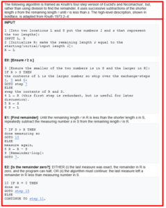
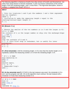
Currently available semantic chunking methods encounter obstacles that the present  implementation cannot overcome. The main challenge lies in segments that are not semantically similar to the surrounding text but are highly relevant to it. Texts containing mathematical formulas, code/algorithm blocks, or quotes are often erroneously chunked due to the presence of these elements in the text, as the embeddings of these fragments are significantly different.


Classical semantic chunking typically results in the creation of several chunks (including usually several very short ones, such as individual mathematical formulas) instead of one larger chunk that would better describe the given fragment. This occurs because the currently created chunk will be „terminated” when it encounters the first fragment that is semantically different from chunk’s content.


Semantic double-pass merging


The issues described above led to the development of the chunking algorithm called “semantic double-pass merging”. Its first part resembles classical semantic chunking (based on mathematical measures such as percentile/standard deviation). What sets it apart is an additional second pass that allows merging of previously created chunks into larger and hence more content-rich chunks. During the second pass, the algorithm looks „ahead” two chunks. If the examined chunk has sufficient cosine similarity with the second next chunk it sees, it will merge all three chunks (the current chunk and the two following ones), even if the similarity between the examined chunk and the next one is low (it could be textually dissimilar but still semantically relevant). This is particularly useful when the text contains mathematical formulas, code/algorithm block, or quotes that may „confuse” the classical semantic chunking algorithm, which only checks similarities between neighboring sentences.


Algorithm

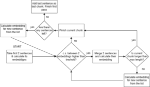
The first part (and the first pass) of the algorithm is a classical semantic chunking method: perform the following steps until there are no more sentences available:

  1. Split the text into sentences.
  2. Calculate cosine similarity (c.s.) for the first two available sentences.
  3. If the cosine similarity value is above the initial_threshold, then merge those sentences into one chunk. Else the first sentence becomes a standalone chunk and return to step 2 with the second sentence and the subsequent one.
  4. If reached the maximum allowable length, stop its growth and proceed to step 2 with the two following sentences.
  5. Calculate cosine similarity between the last two sentences of the existing chunk and the next sentence.
  6. If the cosine similarity value is above the appending_threshold, add the next sentence to the existing chunk and return to step 4.
  7. Finish the current chunk and return to step 2.


Visualization of the first pass of “semantic double-pass merging” method.
Figure 1 – Visualization of the first pass of “semantic double-pass merging” method.


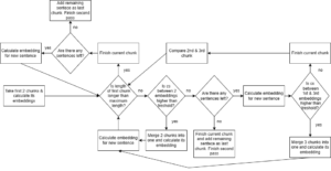
To address scenarios where individual sentences, such as quotations or mathematical formulas embedded within coherent text, pose challenges during semantic chunking, a secondary pass of semantic chunking is conducted.

  1. Take the first two available chunks.
  2. Calculate cosine similarity between those chunks.
  3. If the value exceeds the merging_threshold, then two chunks are merged, ensuring that the length of these chunks does not exceed the maximum allowable length. Then take the next available chunk and return to step 2. If the length does exceed the limit then finish the current chunk and return to step one with second chunk used in that comparison and next available chunk. Elsewhere move to step 4.
  4. Take next available chunk and calculate cosine similarity between first examined chunk and the new (third in that examination) one.
  5. If the value exceeds the merging_threshold, then three chunks are merged, ensuring that the length of these chunks does not exceed the maximum allowable length. Then take the next available chunk and return to step 2. If the length does exceed the limit then finish the current chunk and return to step one with second and third chunk used in that comparison.


If the cosine similarity from the fifth step exceeds the merging threshold, it indicates that the middle-examined chunk was a „snippet” (possibly a quote/mathematical formula/pseudocode) with different embedding values from its surroundings, but still a semantically significant part of the text. This transition ensures that the resulting chunks will be semantically similar and will not be interrupted at inappropriate points, thus preventing information loss.


Visualization of the second pass of “semantic double-pass merging” method.

Figure 2 – Visualization of the second pass of “semantic double-pass merging” method.


Parameters

Thresholds in the algorithm control the grouping of sentences into chunks (in the first pass) and chunks into larger chunks (in the second pass). Here’s a brief overview of the three thresholds:

  • initial_threshold: Specifies the similarity needed for initial sentences to form a new chunk. A higher value creates more focused chunks but may result in smaller chunks.
  • appending_threshold: Determines the minimum similarity required for adding sentences to an existing chunk. A higher value promotes cohesive chunks but may result in fewer sentences being added.
  • merging_threshold: Sets the similarity level for merging chunks. Higher value consolidates related chunks but risks merging unrelated ones.


For optimal performance, set the appending_threshold and merging_threshold relatively high to ensure cohesive and relevant chunks, while keeping the initial_threshold slightly lower to capture a broader range of semantic relationships. Adjust these thresholds based on text characteristics and desired chunking outcomes. Additionally, examples should be added: monothematic text should have higher merging_threshold and appending_threshold in order to differentiate chunks, even if the text is highly related, and to avoid classifying the entire text as a single chunk.


Comparative analysis

The comparative analysis of key chunking methods were conducted in the following environment:

  • Python 3.10.12
  • nltk 3.8.1
  • spaCy 3.7.4 with embeddings model: en_core_web_md
  • LangChain 0.1.11


For the purpose of comparing chunking algorithms, we used LangChain’s SpacyTextSplitter for token-based chunking and sent_tokenize function provided by nltk for sentence-based chunking. After using sent_tokenize, the chunks were created by grouping them according to a predetermined number of sentences. The proposition-based chunking was performed using various OpenAI GPT language models. For semantic chunking with percentile breakpoint LangChain implementation was used.


Case #1: Simple short text

The first test involved assessing how specific models perform (or not) with a simple example where topic change is very distinct. However, the description of each of the three topics consisted of a different number of sentences. Parameters for both token-based chunking and sentence-based chunking were set so that the first topic is correctly classified.

To conduct the test, the following methods along with their respective parameters were used:

  • Token-based chunking: LangChain’s CharacterTextSplitter using tiktoken
    • Tokens in chunk: 80
    • Tokenizer: cl100k_base
  • Sentence-based chunking: 4 sentences per chunk
  • Clustering with k-means: sklearn’s KMeans:
    • Number of clusters: 3
  • Semantic chunking percentile-based: LangChain implementation of SemanticChunker with percentile breakpoint with values for breakpoint 50/60/70/80/90
  • Semantic chunking double-pass merging:
    • initial_threshold: 0.7
    • appending_threshold: 0.8
    • merging_treshold: 0.7
    • spaCy model: en_core_web_md


A picture illustrating token-based chunking, displaying how text is segmented into manageable tokens or chunks.

Figure 3 – Token-based chunking.


 picture illustrating sentence-based chunking, showing how text is divided into individual sentences,

Figure 4 – Sentence-based chunking.


Both token-based and sentence-based chunking encounter the same issue: they fail to detect when the text changes its topic. This can be detrimental for RAGs when „mixed” chunks arise, containing information about completely different topics but connected because these pieces of information happened to occur one after the other. This may lead to erroneous responses generated by the RAG.


A picture illustrating chunking with k-means clustering, showing how text is grouped into clusters based on similarity.

Figure 5 – Chunking with k-means clustering.


The above image excellently illustrates why clustering methods should not be used for chunking. This method loses the order of information. It’s evident here that information from different topics intertwines within different chunks, causing the RAG using this chunking method to contain false information, consequently leading to erroneous responses. This method is definitely discouraged.


Diagram illustrating LangChain's semantic chunking with breakpoint_type set to percentile (breakpoint = 60),

Figure 6 – LangChain’s semantic chunking with breakpoint_type set as percentile (breakpoint = 60).


Typical semantic chunking struggles to perfectly segment the given example. Various values of the breakpoint parameter were tried, yet none achieved perfect chunking.


Semantic chunking with double-pass mergingafter first pass of the algorithm.

Figure 7 – Semantic chunking with double-pass mergingafter first pass of the algorithm.


The primary goal of the first pass of the double-pass algorithm is to accurately identify differences between topics and only connect the most obvious sentences together. In the above visualization, it is evident that no mini-chunk contains information from different topics.


A pictures shows semantic chunking with double-pass merging after second pass of the algorithm.

Figure 8 – Semantic chunking with double-pass merging after second pass of the algorithm.


The second pass of the double-pass algorithm correctly combines previously formed mini-chunks into final chunks that represent individual topics. As seen in the above example, the double-pass merging algorithm handled this simple example exceptionally well.


Case #2: Scientific short text

The next test was to examine how a text containing pseudocode would be divided. The embeddings of pseudocode snippets would significantly differ from the embeddings of text snippets that cut through them. Ultimately, the text and its description should be combined into one chunk to maintain coherence. For this purpose, a fragment of text from Wikipedia about the Euclidean algorithm was chosen. In this comparison, the focus was on juxtaposing semantic chunking methods, namely classical semantic chunking, double-pass, and propositions-based chunking:

  • Semantic chunking percentile-based: LangChain implementation of SemanticChunker with percentile breakpoint set to 60/99/100
  • Proposition-based chunking using gpt-4
  • Semantic chunking double-pass merging:
    • initial_threshold: 0.6
    • appending_threshold: 0.7
    • merging_threshold: 0.6
    • spaCy model: en_core_web_md


A picture shows semantic chunking with percentile breakpoint set at 99.

Figure 9 – Semantic chunking with percentile breakpoint set at 99.


Semantic chunking using percentiles was unable to comprehend the text as a single chunk. The entirety of the sample text was merged into one chunk only when the breakpoint value was set to the maximum value of 100 (which merges all sentences into one chunk).


 A diagram illustrating semantic chunking with a percentile breakpoint set at 60, demonstrating how text is divided into segments based on semantic meaning.

Figure 10 – Semantic chunking with percentile breakpoint set at 60.


Semantic chunking using percentiles with a breakpoint set to 60, which allows for distinguishing between sentences on different topics, struggles with this example. It cuts the algorithm in the middle of a step, resulting in chunks containing fragments of information.


A diagram illustrating semantic double-pass merging chunking, showcasing the process of chunking text in two passes to improve coherence.

Figure 11 – Semantic double-pass merging chunking.


The double-pass merging algorithm performed admirably, interpreting the entire text as a thematically coherent chunk.


A diagram illustrating propositions created by propositions-based chunking, displaying how text is segmented into individual propositions or statements,

Figure 12 – Propositions created by propositions-based chunking.


A diagram showing chunks created by propositions-based chunking, highlighting how text is divided into distinct propositions,
Figure 13 – Chunk created by propositions-based chunking.


The proposition-based chunking method first creates a list of short sentences describing simple facts and then constructs specific chunks from them. In this case, the method successfully created one chunk, correctly identifying that the topic is uniform.


Case #3: Long text

To assess how different chunking methods perform on longer text, the well-known 'PaulGrahamEssayDataset’ available through LlamaIndex was utilized. Subsequently, simple RAGs were constructed based on the created chunks. Their performance was evaluated using the RagEvaluatorPack provided by LlamaIndex. For each RAG, the following metrics were calculated based on 44 questions provided by LlamaIndex datasets:

  • Correctness: This evaluator depends on reference answer to be provided, in addition to the query string and response string. It outputs a score between 1 and 5, where 1 is the worst and 5 is the best, along with a reasoning for the score. Passing is defined as a score greater than or equal to the given threshold. More information here.
  • Relevancy: Measures if the response and source nodes match the query. This metric is tricky: it performs best when the chunks are relatively short (and, of course, correct), achieving the highest scores. It’s worth keeping this in mind when applying methods that may produce longer chunks (such as semantic chunking methods), as they may result in lower scores. The language model checks the relationship between source nodes and response with the query, and then a fraction is calculated to indicate what portion of questions passed the test. The range of this metric is between 0 and 1.
  • Faithfulness: Measures if the response from a query engine matches any source nodes which is useful for measuring if the response is hallucinated. If the model determines that the question (query), context, and answer are related, then the question is counted as 1, and a fraction is calculated to represent what portion of test questions passed the test. The range of values for faithfulness is from 0 to 1.
  • Semantic similarity: Evaluate the quality of a question answering system by comparing the similarity between embeddings of the generated answer and the reference answer. The value of this metric ranges between 0 and 1. Read more about this method here.


More detailed definitions of faithfulness and relevancy metrics are described in this article.


To conduct this test, the following models were created:

  • Token-based chunking: LangChain’s CharacterTextSplitter using tiktoken
    • Tokens in chunk: 80
    • Tokenizer: cl100k_base
  • Sentence based: chunk size is set to 4 sentences,
  • Semantic percentile-based: Langchain’s SemanticChunker with percentile_breakpoint set to 0.65,
  • Semantic double-pass merging:
    • initial_threshold: 0.7
    • appending_treshold: 0.6,
    • merging_treshold: 0.6,
    • spaCy model: en_core_web_md
  • Propositions-based: using gpt-3.5-turbo/gpt-4-turbo/gpt-4 in order to create propositions and chunks. The code is based on the implementation proposed by Greg Kamradt.


For comparison purposes, the average time and costs of creating chunks (embeddings and LLM cost) were juxtaposed. The obtained chunks themselves were also compared. Their average length in characters and tokens was checked. Additionally, the total number of tokens obtained after tokenizing all chunks was counted. The cl100k_base tokenizer was used to calculate the total token count and the average number of tokens per chunk.


Chunking method Average chunking duration Average chunk length
[characters]
Average chunk length
[tokens]
Total token count Chunking cost
[USD]
Token-based 0.08 sec 458 101 16 561 <0.01
Sentence-based 0.02 sec 395 88 16 562 0
Semantic percentile-based 8.3 sec 284 63 16 571 <0.01
Semantic double-pass merging 16.7 sec 479 106 16 558 0
Proposition-based using gpt-3.5-turbo 9 min 58 sec 65 14 2 457 0.29
Proposition-based using gpt-4-turbo 1 h 43 min 30 sec 409 85 6 647 17.8
Proposition-based using gpt-4 40 min 38 sec 548 117 5 987 29.33


As we can see, classical chunking methods operate significantly faster than methods attempting to detect semantic differences. This is, of course, due to the higher computational complexity of semantic chunking algorithms. When looking at chunk length, we should focus on comparing two semantic methods used in the comparison. Both token-based and sentence-based methods have rigid settings regarding the length of created chunks, so comparing their results in terms of chunk length won’t be very useful. Chunks created by classical semantic chunking using percentiles are significantly shorter (both in terms of the number of characters and the number of tokens) than chunks created by semantic double-pass merging chunking.


In this test, no maximum chunk length was set in the double-pass merging algorithm. As a result of tokenization on the created chunks, the sum of tokens in each tested approach turned out to be very similar (except for the proportion-based approach). It’s worth noting the chunks generated by the proposition-based method. The use of the gpt-4 and gpt-4-turbo models results in a significantly longer process time for a single document. As a result of this extended process, the longest chunks are created, but there are relatively few of them in terms of the total number of tokens. This occurs because this approach compresses information by strictly focusing on facts. On the other hand, the propositions-based approach based on gpt-3.5 generates significantly fewer propositions, which then need to be stitched together into complete chunks. As a result, the execution time is much shorter.


The differences in the time required for proposition-based chunking with various models stem from the number of propositions generated by each model. gpt-3.5-turbo created 238 propositions, gpt-4-turbo created 444, and gpt-4 created 361. Propositions generated by gpt-3.5-turbo were also simpler and contained individual facts from multiple domains, making it harder to combine them into coherent chunks, hence the lower average chunk length. Propositions generated by gpt-4-turbo and gpt-4 were more specific and numerous, facilitating the creation of semantically cohesive chunks.


When comparing costs, it’s worth emphasizing that the text used for testing various methods consisted of 75 042 characters. Creating chunks for such a text is possible for free with semantic chunking methods like double-pass (uses spaCy to compute embeddings, and using a different embedding calculation method may increase costs) and classical sentence-based chunking. Methods utilizing embeddings (token-based and semantic percentile-based chunking) incurred costs lower than 0.01 USD. However, significant costs arose with the proposition-based chunking method: the approach using gpt-3.5-turbo costed 0.29 USD. This is nothing compared to generating chunks using gpt-4-turbo and gpt-4, which incurred costs of 17.80 and 29.33 USD, respectively.


Chunking type Mean correctness score Mean relevancy score Mean faithfulness score Mean semantic
similarity score
Token-based 3,477 0,841 0,977 0,894
Sentence-based 3,522 0,932 0,955 0,893
Semantic percentile 3,420 0,818 0,955 0,892
Semantic double-pass merging 3,682 0,818 1,000 0,905
Propositions-based gpt-3.5-turbo 2,557 0,409 0,432 0,839
Propositions-based gpt-4-turbo 3.125 0.523 0.682 0.869
Propositions-based gpt-4 3,034 0,568 0,887 0,885


We can see that the semantic double-pass merging chunking algorithm achieves the best results for most metrics. Particularly significant is its advantage over classical semantic chunking (semantic percentile) as it represents an enhancement of this algorithm. The most important statistic is the mean correctness score, and it is on this metric that the superiority of the new approach is evident.


Surprisingly, the proposition-based chunking methods achieved worse results than the other methods. RAG based on chunks generated with the help of gpt-3.5-turbo turned out to be very weak in the context of the analyzed text, as seen in the above table. However, RAGs based on chunks created using gpt-4-turbo/gpt-4 proved to be more competitive, but still fell short compared to the other methods. It can be concluded that chunking methods based on propositions are not the best solution for long prose texts.


Summary

Applying different chunking methods to texts with diverse characteristics allows us to draw conclusions about each method’s effectiveness. From the test involving chunking a straightforward text with distinct topic segments, it’s evident that clustering-based chunking is totally unsuitable as it loses sentence order. Classical chunking methods like sentence-based and token-based struggle to properly divide the text when segments on different topics vary in length. Classical semantic chunking performs better but still fails to perfectly chunk the text. Semantic double-pass merging chunking flawlessly handled the simple example.


Chunking a text containing pseudocode focused on comparing semantic chunking methods: percentile-based, double-pass, and proposition-based. Semantic chunking with a breakpoint set by percentiles couldn’t chunk the text optimally for any breakpoint value. Even for values allowing chunking of regular text (i.e., settings like in the first test), the method struggled, creating new chunks in the middle of pseudocode fragments. Semantic double-pass merging and propositions-based chunking using gpt-4 performed admirably, creating thematically coherent chunks.


A test conducted on a long prose text primarily focused on comparing metrics offered by LlamaIndex, revealing statistical differences between methods. Semantic double-pass merging and proposition-based method using gpt-4 generated the longest chunks. The fastest were classical token-based and sentence-based chunking due to their low computational requirements. Next were the two semantic chunking algorithms: percentile-based and double-pass chunking, which took twice as long. Proposition-based chunking took significantly longer, especially when using gpt-4 and gpt-4-turbo. This method, using these models, also incurred significant costs.


The free tested chunking methods were sentence-based and semantic double-pass merging chunking. Nearly cost-free methods were those based on token counting: token-based chunking and semantic percentile-based chunking. Comparing statistical metrics for RAGs created based on chunks generated by the aforementioned methods, semantic double-pass merging chunking performs best in most statistics. It’s notable that double-pass outperformed regular semantic percentile-based chunking as it’s its enhanced version. Classical chunking methods performed averagely, but far-reaching conclusions cannot be drawn about them because the optimal chunk length may vary for each text, drastically altering metric values. Proposition-based chunking is entirely unsuitable for chunking longer prose texts. It statistically performed the worst, taking significantly longer and being considerably more expensive.


All content in this blog is created exclusively by technical experts specializing in Data ConsultingData InsightData Engineering, and Data Science. Our aim is purely educational, providing valuable insights without marketing intent.

bg

Chunking methods in RAG: comparison

Learn how to pick best textual data chunking method to lower processing costs and maximize efficiency!

Read more arrow

Introduction


In today’s digital landscape, the management and analysis of textual data have become integral to numerous fields, particularly in the context of training language models like Large Language Models (LLMs) for various applications. Chunking, a fundamental technique in text processing, involves splitting text into smaller, meaningful segments for easier analysis.


While traditional methods based on token and sentence counts provide initial segmentation, semantic chunking offers a more nuanced approach by considering the underlying meaning and context of the text. This article explores the diverse methodologies of chunking and aims to guide readers in selecting the most suitable chunking method based on the characteristics of the text being analyzed. The importance of this is particularly evident when utilizing LLMs to create RAGs (Retrieval-Augmented Generative models). Additionally, it dives into the intricacies of semantic chunking, highlighting its significance in segmenting text without relying on LLMs, thereby offering valuable insights into optimizing text analysis endeavors.


Understanding Chunking


Chunking, in its essence, involves breaking down a continuous stream of text into smaller, coherent units. These units, or „chunks,” serve as building blocks for subsequent analysis, facilitating tasks such as information retrieval, sentiment analysis, and machine translation. The effectiveness of chunking is particularly important in crafting RAG (Retrieval-Augmented Generation) models, where the quality and relevance of the input data significantly impact model performance. This happens because different embedding models have different maximum input lengths. While conventional chunking methods rely on simple criteria like token or sentence counts, semantic chunking takes a deeper dive into the underlying meaning of the text, aiming to extract semantically meaningful segments that capture the essence of the content.


Key concepts


Before diving into the main body of the article, it’s worth getting to know a few definitions/concepts.


Text embeddings

Text embeddings are numerical representations of texts in a high-dimensional space, where texts with similar meanings are closer to each other. In this space, each dimension corresponds to a word or token from the vocabulary. These representations capture semantic relationships between texts, allowing algorithms to understand language semantics.


An illustration showcasing word embeddings, featuring representations of a man, woman, queen, and king, 
Figure 1 Word embeddings - Source.


Cosine similarity

Cosine similarity is a measure frequently employed to assess the semantic similarity between two embeddings. It operates by computing the cosine of the angle between two vector embeddings that represent these sentences in a high-dimensional space. These vectors can be represented in 2 ways:


You can find more information about the differences between sparse and dense vectors here. This similarity measure evaluates the alignment or similarity in direction between the vectors, effectively indicating how closely related the semantic meanings of the sentences are. A cosine similarity value of 1 suggests perfect similarity, implying that the semantic meanings of the sentences are identical, while a value of 0 indicates no similarity between the sentences, signifying completely dissimilar semantic meanings. Additionally, an exemplary calculation along with an explanation is well presented in following video.


A sample visualization demonstrating cosine similarity in a two-dimensional space.

                             Figure 2 Sample visualization of cosine similarity - Source.


LLM’s context window

In Language Modeling (LLM), a context window refers to a fixed-size window that is used to capture the surrounding context of a given word or token in a sequence of text. This context window defines the scope within which the model analyzes the text to predict the next word or token in the sequence. By considering the words or tokens within the context window, the model captures the contextual information necessary for making accurate predictions about the next element in the sequence. It’s important to note that various chunking methods may behave differently depending on the size and nature of the context window used. The size of the context window is a hyperparameter that can be adjusted based on the specific requirements of the language model and the nature of the text data being analyzed. For more information about context window check this article.


A sample visualization illustrating a context window in natural language processing

Figure 3 Sample visualization of context window - Source.


Conventional chunking methods


Among chunking methods, two main subgroups can be identified. The first group consists of conventional chunking methods, which split the document into chunks without considering the meaning of the text itself. The second group consists of semantic chunking methods, which divide the text into chunks through semantic analysis of the text. The diagram below illustrates how to distinguish between various methods


A diagram illustrating the differences between selected types of chunking in natural language processing

Figure 4. Diagram representing the difference between the selected types of chunking.


Source-text-based chunking

Source-text-based chunking involves dividing a text into smaller segments directly based on its original form, disregarding any prior tokenization. Unlike token-based chunking, which relies on pre-existing tokens, source-text-based chunking segments the text purely based on its raw content. This method allows for segmentation without consideration of word boundaries or punctuation marks, providing a more flexible approach to text analysis. Additionally, source-text-based chunking can employ a sliding window technique.


This involves moving a fixed-size window across the original text, segmenting it into chunks based on the content within the window at each position. The sliding window approach facilitates sequential segmentation of the text, capturing local contextual information without relying on predefined token boundaries. It aims to capture meaningful units of text directly from the original source, which may not necessarily align with token boundaries. However, a drawback is that language models typically operate on tokenized input, so text divided without tokenization may not be an optimal solution.


It’s worth mentioning that LangChain has a class named CharacterTextSplitter, which might suggest splitting text character by character. However, this is not the case, as this function splits the text based on the regex provided by the user (e.g., by space or newline characters). This is because each splitter in LangChain inherits from the text_splitter class, which takes chunk_size and overlap as arguments. Subclasses override the split_text method in a way that may not utilize the parameters contained in the base class.


Token-based chunking

Token-based chunking is a text processing method where a continuous stream of text is divided into smaller segments using predetermined criteria based on tokens. Tokens, representing individual units of meaning like words or punctuation marks, play a crucial role in this process. In token-based chunking, text segmentation occurs based on a set number of tokens per chunk. An important consideration in this process is overlapping, where tokens may be shared between adjacent chunks.


However, when chunks are relatively short, significant overlap can occur, leading to a higher percentage of repeated information. This can result in increased indexing and processing costs for such chunks. While token-based chunking is straightforward and easy to implement, it may overlook semantic nuances due to its focus on token counts rather than the deeper semantic structure of the text. Nonetheless, managing overlap is essential to balance the trade-off between segment coherence and processing efficiency. This function is built into popular libraries LlamaIndex and LangChain.


Sentence-based chunking

Sentence-based chunking is a fundamental approach in text processing that involves segmenting text into meaningful units based on sentence boundaries. In this method, the text is divided into chunks, with each chunk encompassing one or more complete sentences. This approach leverages the natural structure of language, as sentences are typically coherent units of thought or expression. Sentence-based chunking offers several advantages, including facilitating easier comprehension and analysis by ensuring that each chunk encapsulates a self-contained idea or concept. Moreover, this method provides a standardized and intuitive way to segment text, making it accessible and straightforward to implement across various text analysis tasks.


However, sentence-based chunking may encounter challenges with complex or compound sentences, where the boundaries between sentences are less distinct. In such cases, the resulting chunks may vary in length and coherence, potentially impacting the accuracy and effectiveness of subsequent analysis. Despite these limitations, sentence-based chunking remains a valuable technique in text processing, particularly for tasks requiring a clear and structured segmentation of textual data. Sample implementation is available in nltk.tokenize.


Recursive chunking

Recursive chunking is a text segmentation technique that employs either token-based or source-text-based chunking to recursively divide a text into smaller units. In this method, larger chunks are initially segmented using token-based or source-text-based chunking techniques. Then, each of these larger chunks is further subdivided into smaller segments using the same chunking approach. This recursive process continues until the desired level of granularity is achieved or until certain criteria are met. Its drawback is computational inefficiency.


Hierarchical chunking

Hierarchical chunking is an advanced text segmentation technique that considers the complex structure and hierarchy within the text. Unlike traditional segmentation methods that divide the text into simple fragments, hierarchical chunking examines relationships between different parts of the text. The text is divided into segments that reflect various levels of hierarchy, such as sections, subsections, paragraphs, sentences, etc. This segmentation method allows for a more detailed analysis and understanding of the text structure, which is particularly useful for documents with complex structures such as scientific articles, business reports, or web pages.


Hierarchical chunking enables the organization and extraction of key information from the text in a logical and structured manner, facilitating further text analysis and processing. An advantage of hierarchical chunking is its ability to effectively group text segments, particularly in well-formatted documents, enhancing readability and comprehension. However, a drawback is its susceptibility to malfunction when dealing with poorly formatted documents, as it relies heavily on the correct hierarchical structure of the text. LangChain comes with many built-in methods for hierarchical chunking, such as MarkdownHeaderTextSplitter, LatexTextSplitter, and HTMLHeaderTextSplitter.


Semantic chunking methods


Semantic chunking is an advanced text processing technique aimed at dividing text into semantically coherent segments, taking into account the meaning and context of words. Unlike traditional methods that rely on simple criteria such as token or sentence counts, semantic chunking utilizes more sophisticated techniques of semantic analysis to extract text segments that best reflect the content’s meaning. To perform semantic chunking, various techniques can be employed. As a result, semantic chunking can identify text segments that are semantically similar to each other, even if they do not appear in the same sentence or are not directly connected.


Clustering with k-means

Semantic chunking using k-means involves a multi-step process. Firstly, sentence embeddings need to be generated using an embedding model, such as Word2Vec, GloVe, or BERT. These embeddings represent the semantic meaning of each sentence in a high-dimensional vector space. Next, the k-means clustering algorithm is applied to these embeddings to group similar sentences into clusters. Implementing semantic chunking with k-means requires a pre-existing embedding model and expertise in NLP and machine learning. Additionally, selecting the optimal number of clusters (k) is challenging and may necessitate experimentation or domain knowledge.


One significant drawback of this approach is the potential loss of sentence order within each cluster. K-means clustering operates based on the similarity of sentence embeddings, disregarding the original sequence of sentences. Consequently, the resulting clusters may not preserve the chronological or contextual relationships between sentences. We strongly advise against using this method for text chunking when constructing RAGs. It leads to the loss of meaning in the processed text and may result in the retriever returning inaccurate content.


Propositions-based chunking

This chunking strategy explores leveraging LLMs to discern the optimal content and size of text chunks based on contextual understanding. At the beginning, the process involves creating so-called “propositions”, often facilitated by tools like LangChain. Propositions are defined as atomic expressions within text, each encapsulating a distinct factoid and presented in a concise, self-contained natural language format.


These propositions are then passed to an LLM, which determines the optimal grouping of propositions based on their semantic coherence. Performance of this approach heavily depends on the language model the user chooses. Despite its effectiveness, a drawback of this approach is the high computational costs incurred due to the utilization of LLMs. Extensive explanation of this method is in this article and a modified proposal is presented in this tweet.


Standard deviation/percentile/interquartile merging

This semantic chunking implementation utilizes embedding models to determine when to segment sentences based on differences in embeddings between them. It operates by identifying differences in embeddings between sentences, and when these differences exceed a predefined threshold, the sentences are split. Segmentation can be achieved using percentile, standard deviation, and interquartile methods. A drawback of this approach is its computational complexity and the requirement for an embedding model. This algorithm’s implementation is available in LlamaIndex. Greg Kamradt showcased this idea in one of his tweets.


Double-pass merging (our proposal)

Considering the challenges faced by semantic chunking using various mathematical measures (standard deviation/percentile/interquartile), we propose a new approach to semantic chunking. Our approach is based on cosine similarity, and the initial pass operates very similarly to the previously described method. What sets it apart is the application of a second pass aimed at merging chunks created in the first pass into larger ones. Additionally, our method allows for looking beyond just the nearest neighbor chunk.


This is important when the text, which may be on a similar topic, is interrupted with a quote (which semantically may differ from the surrounding text) or a mathematical formula. The second pass examines two consecutive chunks: if no similarity is observed between the two neighbors, it checks the similarity between the first and third chunks being examined. If these two chunks are classified as similar, then all three chunks are merged into one. A detailed description of the algorithm and code will be presented in an upcoming article, which will be published shortly.


Summary

As you can see there are many diverse chunking algorithms differing in various aspects such as required computational power, costs, duration, and implementation complexity. Selection of an appropriate chunking algorithm is an important decision as it impacts two key factors of the solution: quality of final results (quality of answers generated by RAG) and cost of running it. Therefore, it should be preceded by a thorough analysis of, amongst others, the purpose for which the chunking is to be performed and quality of source documents. Our next article comparing the performance of various chunking methods can be helpful with taking a decision. Stay tuned!


All content in this blog is created exclusively by technical experts specializing in Data ConsultingData InsightData Engineering, and Data Science. Our aim is purely educational, providing valuable insights without marketing intent.

bg

Chunking methods in RAG: overview of available solutions

Explore available chunking methods and how they work!

Read more arrow

Intro


In the world of data science and technology, one cannot ignore the allure of Large Language Models (LLMs). Their capabilities are undeniably captivating for enthusiasts in the field. However, despite the excitement, caution should be exercised. Let’s talk about when it’s not advisable to use LLMs in your data science projects.


Targeted use case and limited data


As we all know, Large Language Models are trained on a massive amount of data so that they can perform a variety of tasks, allowing users to save a significant amount of time. They provide higher-quality outputs in tasks like translation, text generation, and question answering, compared to, for example, rule-based systems where developers manually create rules and patterns for language understanding. Conversely, if your data science project involves highly technical or specialized content, using a pre-trained LLM alone may result in inaccurate or incomplete results. In such cases, incorporating domain-specific models or knowledge bases may be necessary. To accomplish this, a substantial amount of data is essential, given that these models possess billions of parameters. Effective fine-tuning requires a significant quantity of data.


Consequently, if there is an awareness that the data available is limited, or if there are constraints on the data, it is advisable to first consider an approach utilizing Natural Language Processing (NLP). In such cases, an NLP model or less complex LLM, which is also known as Small Language Model can still yield satisfactory results on the available dataset. Review our article about the advantages of using SLMs over LLMs: When bigger isn’t always better – Bring your attention to Small Language Models.


Factuality


When discussing the drawbacks of Large Language Models, it is essential to mention one of the most common issues, namely the tendency of models to hallucinate. Anyone who has used or is using ChatGPT3.5 has undoubtedly experienced this phenomenon – simply put, it is the moment when the model’s responses are completely incorrect, containing untrue information, despite appearing coherent and logical at first glance. This is primarily influenced by the dataset on which the model was trained, as it is vast, originating from many sources that often may contain subjective, biased views, or distorted information.


The cause of hallucinations also lies in using models for tasks they were not adapted for. The feature which seems to be an advantage when it comes to creative tasks, such as composing songs and writing poems, becomes a disadvantage when we expect the model to provide only factual information. As we know, LLMs perform very well in general natural language processing tasks, so applying them to specific Data Science tasks will result in outcomes deviating from the truth. In such situations, it is necessary to tailor these models to a specific problem, armed with an adequate amount of high-quality data. As we know from the previous paragraph, acquiring such data is a challenging and laborious process. However, even if we manage to create such a dataset, the issue of fine-tuning the model still remains, posing an additional challenge if computational power and cost resources are limited.


Streaming applications such as multi-round dialogue


LLMs also encounter challenges in processing streaming data. As we know, they are trained on texts of finite length (a few thousand tokens), resulting in a decrease in performance when handling sequences longer than those on which they were trained. The architecture of LLMs caches key-value states of all previous tokens during inference, consuming a significant amount of memory. As a result of this limitation, large language models face difficulties in handling systems that require extended conversations, such as chatbots or interactive systems.


It is worth noting that the StreamingLLM framework comes to the rescue in this context, where the authors leverage the initial tokens of LLMs to serve as the focal point for the allocation of attention scores by caching initial tokens alongside recent ones. Nevertheless, keep in mind that this framework does not extend LLMs context window – retaining only the latest tokens and attention sinks while discarding the middle ones.


Security concerns


Deploying LLMs in data science projects may raise legal and ethical challenges, especially when dealing with sensitive or regulated domains. LLMs can be vulnerable to attacks, where malicious actors intentionally input data to deceive the model. It is crucial to remember that the model’s responses may contain inappropriate or sensitive information.


The absence of proper data filtering or management can lead to the leakage of private data, exposing us to the risk of privacy and security breaches. The recent inadvertent disclosure of confidential information by Samsung employees highlights significant security concerns associated with the use of Large Language Models (LLMs) like ChatGPT. Samsung’s employees accidentally leaked top-secret data while seeking assistance from ChatGPT for work-related tasks.


The incident serves as a stark reminder that any information shared with these models is retained and utilized for further training, raising privacy and data security issues. This incident not only demonstrates the unintentional vulnerabilities associated with using LLMs in corporate settings but also underscores the need for organizations to establish strict protocols to safeguard sensitive data. It emphasizes the delicate balance between leveraging advanced language models for productivity and ensuring robust security measures to prevent inadvertent data leaks.


Interpretability and explainability


Another important aspect is that LLMs generate responses that are non-interpretable and unexplainable. Large Language Models are often referred to as black boxes, as it is often impossible for users or even the creators of the model to determine exactly what factors influenced a particular response. Additionally, there may be cases where the same question yields different answers, which is unacceptable for certain use cases.


Therefore, if project requirements include a transparent and logical decision-making process, relying on responses from a language model is not advisable. However, it is still worth considering eXplainable Artificial Intelligence (XAI) in Natural Language Processing (NLP) for such problems. Explore the role of XAI in addressing the interpretability posed by machine learning models in another of our insightful articles: Unveiling the Black Box: An overview of Explainable AI.


Real-time processing


In situations where project requirements involve processing responses in real-time, large language models are not a suitable choice. They possess an enormous number of parameters, translating into a significant demand for computational power for processing. The computational load of large models can be prohibitive. Due to the high complexity, large language models often exhibit extended inference times, introducing delays that are unacceptable in real-time contexts. Applications processing vast amounts of data in real-time, given their flexibility and the tendency for context changes in text, would require continuous fine-tuning to meet demands. This, in turn, results in substantial costs for maintaining model quality.


Summary


In summary, while large language models exhibit impressive language understanding, their practical implementation comes with challenges related to computational efficiency, latency, resource usage, scalability, unpredictability, interpretability, adaptability to dynamic environments, and the risk of biases. These factors should be carefully considered when deciding whether to use large language models in data science projects.


All content in this blog is created exclusively by technical experts specializing in Data ConsultingData InsightData Engineering, and Data Science. Our aim is purely educational, providing valuable insights without marketing intent.

bg

LLMs in Data Science projects – practical challenges

Large Language Models (LLMs) have amazing language comprehension, but their practical usage can cause challenges related to efficiency, latency, resource usage, scalability and more!

Read more arrow

Intro


Undoubtedly, there is a lot of hype around Large Language Models. We are pleased to observe what is happening and simultaneously gather knowledge and experience in the field. These powerful models have demonstrated their immense capabilities in a wide range of use cases, so our customers are also curious about new possibilities and eager to use in the projects popular large-scale models like ChatGPT. To the surprise of our clients, it is not always the best choice.


In a world where bigger is often perceived as better, perhaps it’s time to challenge this preconception – at least when it comes to Large Language Models. In this article, we’ll delve into scenarios in which opting for a more modestly sized LLM might prove to be the wiser and more pragmatic approach.


Large language models (LLMs) are characterized by a significant increase in the number of parameters they possess, often reaching billions or even trillions. As the parameter count grows, these models tend to deliver greater accuracy and generate higher-quality outputs in tasks like translation, text generation, and question answering. Imagine GPT-3.5, developed by OpenAI, a powerful language model with 175 billion parameters. As the GPT series is expanding the GPT-4 is said to be based on eight models with 220 billion parameters each, which gives a total of about 1.76 trillion parameters, making it nearly 1000 times larger than the GPT-3.5. However, it is important to note that as LLMs grow, they bring along a set of challenges that must be acknowledged and considered.


Cost


The first challenge could be the cost, which depends on many factors. Primarily, LLMs can be distinguished for commercials and open source. In the case of commercial ones usually the cost is evaluated for each model usage based on the number of tokens used in its call. Even if the unit cost of the model usage is relatively small, for example gpt-3.5-turbo around $0.002 per 1000 tokens, the cost grows rapidly if you want to use the model a million times a day.


On the other hand, open-source models have no direct cost per request, they are generally free to use. Open-source LLMs expenses are related to the infrastructure. Simplifying, GPU memory requirements depend linearly on the number of model parameters. It can be assumed that storing a 1B parameter in GPU memory, required for inference — costs 4 GB at 32-bit float precision. Please find below the cost of some open-source models which can be run on the NC A100 v4 series.


Model name Size Cluster GPU Cost
LLaMA2–7B 7b parameter NC24ads A100 v4 1X A100 $3.67/hour
Dolly-v2-12b 12b parameter NC24ads A100 v4 1X A100 $3.67/hour
LLaMA-2–70b 70b parameter NC48ads A100 v4 2X A100 $7.35/hour


Smaller LLMs offer a more efficient alternative, allowing for computing and training on less powerful hardware. Sometimes it is possible to self-host such a model on a private machine instead of using computational server, but we need to be sure to provide minimum system requirements to do so. In the end, the number of requests or the usage volume is a critical factor in determining the real cost for a given use case.


When we think about resources, environmental aspects are also an advantage, as using smaller models creates a smaller carbon footprint.


Use case


Despite the fact that pre-trained LLMs can provide valuable insights and generate text in various domains, they may lack the domain-specific knowledge required for certain specialized tasks. In the realm of data science projects, where the focus is on addressing specific business needs, the relevance of information concerning distinctions between butter and margarine, or the causes of the French Revolution, is not evident. While information from diverse set of areas such as cuisine or history can be insightful, they may not be pertinent to business clients seeking solutions tailored to their specific tasks. Not every project requires the vast knowledge and generative abilities of billion-parameter LLMs.


If your data science project involves highly technical or specialized content, using a pre-trained LLM alone may result in inaccurate or incomplete results. In such cases, incorporating domain-specific models or knowledge bases may be necessary. Smaller models can be tailored to specific use cases more effectively. They allow data scientists to fine-tune the model for particular tasks, resulting in better performance and efficiency.


Response time


Massive models can introduce delays in processing due to their size and complexity. Generally, smaller language models provide responses faster than larger models. This is because smaller models have fewer parameters and require less computational power to generate responses. They can process and generate text more quickly, making them a preferred choice for applications where low latency is important. Let’s see the difference in OpenAI models we mentioned earlier.  One of the experiments comparing response time for these models result in following:

  • GPT-3.5: 35ms per generated token,
  • GPT-4: 94ms per generated token.


The trade-off between response speed and response quality needs to be carefully considered when choosing a model for a specific application. The choice of model size should align with the specific requirements and constraints of the project.


With all that said, we hoped to expand your perspective on the language models and the idea that larger models may not always be a better one. When considering an LLM for your data science project, it’s essential to evaluate the specific requirements of your task and weigh them against the potential drawbacks of using a massive model. Smaller LLMs offer practical advantages in terms of computational efficiency, cost-effectiveness, environmental sustainability, and tailored performance, despite their own disadvantages and limitations.


All content in this blog is created exclusively by technical experts specializing in Data ConsultingData InsightData Engineering, and Data Science. Our aim is purely educational, providing valuable insights without marketing intent.

bg

When bigger isn't always better – taking a look at Small Language Models!

In 2023 LLMs became symbol of AI capability. But they are not always the best solution for your AI needs. Why? Read the article and find out!

Read more arrow

Intro 


Are you considering the implementation of a business intelligence tool but find it challenging to select the right one? There are multiple options available on the market, so the choice might be difficult, as not every piece of information is easily accessible or clear. Additionally small details can have a future impact on scalability, costs or ability to integrate other solutions. But you are in luck as our experts are ready to provide you with guidance and a comparison of three distinct BI systems, to help you make a more informed choice.


Power BI, created by Microsoft, is a very user-friendly business intelligence tool. It enables you to easily import data from various sources and create interactive dashboards as well as reports. Its drag-and-drop interface makes it accessible to non-technical users and allows it to work well in self-service scenarios. Additionally, this tool is also very robust when it comes to enterprise-grade solutions.

Being a part of Microsoft’s ecosystem is one of its strongest points as it seamlessly integrates with the whole suite of Microsoft products like Excel, Power Point, Teams and Azure. It is also a key component in a brand-new data platform called Microsoft Fabric!


Tableau is one of the first players when it comes to BI tooling on the market. It empowers users to explore and understand data through interactive and shareable dashboards. Tableau also supports data integration from multiple sources, offering visually appealing and complex visualizations. The ability to create very sophisticated visualizations which can reveal hidden business insights is Tableau’s most recognizable trademark.

Additionally, this tool encourages collaboration, making it suitable for teams to share insights and work on data projects. Currently owned by Salesforce, it easily integrates with this most popular CRM system on multiple levels.


Wyn Enterprise might be the least known of the three, but it has some unique approach amongst BI tooling.  Let’s start by saying that it is a comprehensive business intelligence and reporting platform designed for enterprise-level data analysis and provides robust data integration capabilities, customizable reporting, and dashboarding options.

It prioritizes security and governance, making it suitable for large organizations with strict data compliance requirements. The main focus of this solution are embedding scenarios for a vast number of users. Combine it with exceptionally attractive licensing and you have a very good combo for many organizations!


Deep dive


Connecting and transforming data:


Let’s explore how the tools stack up when it comes to data preparation, connectivity, automation and scalability.


Having out-of-the-box data connectors and the ability to shape the data is crucial for smooth and effective workflow. This is especially important when working with excel or csv files. But even with database as a source, small tweaks in data are often necessary. A tool that allows the user to quickly connect to particular data sources and transform data to correct format without the need to use other tools is a blessing, increasing the efficiency and easy of use of the whole system.


Well-prepared data is the basis for proper analysis and thus for correct business information. Properly modeled and mapped data can contribute to the correct calculation of key business KPIs.


Looking at Power Bi, typically the first component users interact with is Power Query. And this is great because Power Query can be also found in Excel ( the most popular analytical tool on our planet btw.) and is well known among its users. Power Query is also praised both for its intuitive GUI and for its M language which offers great flexibility for data transformations.


On the other hand, Tableau has its own offering called Tableau Prep which is highly appreciated for its extensive use of AI in suggestions for data transformation processes. This helps the users to speed up work time and take advantage of facilities that he would not have noticed. In addition, most things can be done using a graphical interface, without any code. Wyn Enterprise provides some data preparation options, although in a more limited capacity. So preferably, it would be used with data that is already clean and transformed.


All three tools come equipped with a diverse array of data connectors, ensuring effortless integration with popular databases. They each support both scheduled and incremental refresh options, enabling users to keep their data current. Furthermore, they provide flexibility in selecting various connection types tailored to specific requirements.


A noteworthy feature shared by Tableau and Wyn Enterprise is the absence of any limits on data input size. This means your data can scale in tandem with your business growth, free from constraints. Additionally, all three tools are equipped with incremental refresh capabilities, resulting in efficient data updates and options to parametrize data sources, which greatly improves the experience of working with multiple data environments.

A table comparing Power BI, Tableau, and Wyn Enterprise,


Modelling


Data modeling is one of the key things when working with data. Starting with any work, architects, bi-developers, data engineers and data modelers face the challenge of creating a model that fully meets business requirements. This can be difficult, especially with large and complex models based on different data sources. In this case, we expect that the BI tool supports developer in this task and offers the highest possible data processing performance. So, we would like to compare Tableau, Power BI and Wyn Enterprise applications in the most important aspects for us from the developer’s point of view.


All of the aforementioned software offers the possibility of modeling and creating relationships between tables. They all work best together in the context of efficiency and optimization in the structure of star schema. All of the three tools allow you to create measures prepared for specific business requirements. Power BI and Wyn have very similar analytical languages, with the same concepts such as context and context transition. Although there are some differences in the number of functions available (in favor of Power BI). Tableau offers VizQl which is really similar to SQL language which we use in database. That makes it easier for people switching from a database to BI application.


 A table comparing Power BI, Tableau, and Wyn Enterprise, focusing on their data modeling capabilities. 


Reporting


The reporting layer is very important as it touches both report developers, who create complex dashboards based on gathered requirements, and business stakeholders who use those dashboards on a daily basis. Therefore, reporting capabilities must fulfill the needs of both groups. For developers the tool needs to be flexible, easy to use and with vast amounts of functionality.


Having those attributes results in a data product (report, dashboard) that will be used on a daily basis by the Business and will grant observability, deliver insights or just plainly make their life easier when it comes to running their company.


We can clearly say that in this category Tableau is ahead of the competition. It is following a grammar of graphics approach where visuals can be built layer by layer. Some things that are easily achieved in Tableau are out of reach when using Power Bi or Wyn Enterprise. Power BI is currently investing heavily in its native visuals and its reporting capabilities so we can clearly expect some great features in the coming months. It is also worth mentioning that Wyn Enterprise has more out-of-the-box visuals than Power BI at this moment.


We’ve prepared a detailed comparison of available features:


 A table comparing Power BI, Tableau, and Wyn Enterprise, focusing on their data reporting capabilities,


Sharing of data products / Administration


The ability to share reports, manage access and allow users to see only the relevant data is basically the main difference that distinguishes BI tools from non-BI ones, such as MS Excel. In the world of Excel, spreadsheets can be sent or shared without any restrictions. Typically, users can modify the data, perform their own detailed analysis and suddenly what happens is that we have multiple versions of the same file flying around and nobody knows which one is the right one. A true nightmare.


With BI systems like Power BI, Tableau or Wyn Enterprise it should not happen as those tools have built-in sharing functionalities, access management, security, data loss prevention and many more. Business users wouldn’t be able to modify the underlying data but will be able to perform their own analysis using available models. Perfect!


The second thing that is worth keeping an eye on is what happens with your data assets, as they are crucial to get the most out of your BI solutions. Let’s imagine a real-life situation. You worked hard to ingest all the relevant data, transformed it, modeled it by applying all the hard gathered business logic, created splendid dashboards and you think you can rest now?


Well, not really… Truth is that there might be a possibility that end-users are not using your data product as it doesn’t bring them any kind of business value. To know that it is the case and to react quickly by adjusting final solution you need to have some observability of what is going on. You would like to monitor usage rates and also get relevant feedback from end users.


A table comparing Power BI, Tableau, and Wyn Enterprise, emphasizing their capabilities for sharing data products and administration features,


Development & Ecosystem


A table comparing Power BI, Tableau, and Wyn Enterprise, focusing on their development and ecosystem features


AI


AI! The new word of the year. If you are not sleeping under a rock, then you know we couldn’t omit it in our analysis. AI-based solutions are being added to almost every tool to increase development speed and/or increase user experience. AI features can be divided into the ones that use simpler ML algorithms and the ones based on modern Large Language Models.


The first group has been available in many BI tools for several years – mainly in the form of more sophisticated charts that could reveal some hidden insights or as interface where users could ask the question about data (with really mixed results). The second group is being introduced as we speak.


It brings the promise of huge productivity boost for both report developers and business users. Available previews show that LLMs could help developers with building report elements, generating code and performing deeper analysis. Business users would be able to ask questions about data, receive report summaries or insights-based recommendations.


The changes are both rapid and promising, so it is important to watch out for new tools and implementations. But for now, let’s focus on the comparison of existing features

Both Microsoft and Salesforce are heavily investing in this domain so in Power BI we will have Copilot serving both developers and users and in Tableau we will have Einstein Copilot (for developers) and Tableau Pulse (for business users).


 A table comparing Power BI, Tableau, and Wyn Enterprise, highlighting their AI capabilities,


As you can see, each solution has its strengths. The choice is not easy and should always take into consideration needs, means and perspectives of an organizations. But with our guide (that you can always go back to!) You should be able to decide on the path that will result in highest efficiency and scalability, as well as lowest costs!


All content in this blog is created exclusively by technical experts specializing in Data ConsultingData InsightData Engineering, and Data Science. Our aim is purely educational, providing valuable insights without marketing intent.

bg

Unlocking Data Insights with Power BI, Tableau, and Wyn Enterprise

Are you considering the implementation of a business intelligence tool but find it challenging to select the right one?? Read the article and be learn a Bit about possible tools, their characteristics and comparisons!

Read more arrow

Understanding dbt project structure for quality assurance


In this comprehensive guide, we delve into the critical realm of data quality assurance using dbt (data build tool). Data quality is paramount in the world of data analytics and decision-making. To ensure the reliability, accuracy, and consistency of your data models, you need a robust testing framework and a well-organized project structure.


Here are the key files and directories you’ll be working with in a dbt project:


  • yml: Located in the ~/.dbt/ or %USERPROFILE%\.dbt\ directory, this file contains your database connection settings. It allows you to set up multiple profiles for different projects or environments
  • models: This directory contains your data models or SQL transformation files. Each file represents a single transformation, such as creating tables, views, or materialized views.
  • macros: Macros are reusable pieces of SQL code that can referenced in your models. You can store generic tests here or in tests/generics folders.
  • snapshots: The snapshots directory which contains snapshot files that define how to capture the state of specific tables in your database over time.
  • tests: directory in which you can store test SQL files for your data models. These tests help ensure data quality and consistency.
  • seeds: Seeds are essentially CSV or TSV files containing raw data. dbt loads these static data files into tables in your specified schema. Seeds can contain sample data used for testing your dbt models or other data processing logic.
  • analyses: The analysis directory contains ad-hoc SQL files for exploring data and performing data analysis.
  • target: Directory automatically created by dbt when you run the dbt run command. It contains the compiled and executed SQL code from your models. It is useful when debugging the pipeline.


By understanding the key files and directories in your dbt project, you can effectively organize, manage, and scale your data transformation processes while ensuring data quality in your project.


Overview of dbt’s testing framework


Dbt’s testing framework is designed to ensure data quality and consistency by validating the data within your models. It provides built-in tests, as well as the ability to create custom tests tailored to your specific data requirements. The testing framework is an essential component of any dbt project as it promotes trust in your data and helps identify issues early in the development process.


dbt’s testing framework includes the following components:


Generic Tests:

These are predefined tests that validate the structure of your data. Initially, there are four of them but you can create and add more. The initial four are:

  • unique: Ensures that a specified column has unique values.
  • not_null: Checks that a specified column does not contain null values.
  • accepted_values: Validates that a column contains only specified values.
  • relationships: Ensures that foreign key relationships between tables are consistent.


You can configure generic tests in the schema.yml file which is associated with your models.


Custom Data Tests:

Custom data tests allow you to define your own SQL queries to test specific data requirements not covered by generic tests. These tests are written in individual SQL files and stored in the tests directory of your dbt project. When creating custom data tests, ensure the SQL query returns zero rows for a successful test or one or more rows for a failed test.


Test Configuration:

dbt allows for configuration of your tests by setting test severity levels, adjusting error thresholds, or even disabling specific tests. These configurations can be defined in the dbt_project.yml file or directly within the schema.yml file for individual tests.


Test Execution:

To execute tests in dbt, use the dbt test command. This command runs all the tests defined in your project, including schema, and custom data tests. The results are displayed in the console, indicating the success or failure of each test, along with any relevant error messages.


Test Documentation:

dbt 's testing framework also integrates with other feature. When generating documentation for your project, the test information is included in the generated documentation, providing a comprehensive overview of quality checks performed on your data models.


By integrating data tests into your development workflow, dbt’s testing framework empowers you to actively safeguard the reliability and accuracy of your data models. This proactive approach ensures that potential data issues are identified and rectified early in the development process, preventing inaccuracies and inconsistencies from proliferating through your data pipeline. As a result, you can trust that your data models consistently produce high-quality, dependable insights crucial for informed decision-making.


Tips for setting up your testing environment


Setting up a testing environment for your dbt project is crucial to ensure data quality and integrity. Here are some tips to help you create an efficient and effective testing environment:


  • Use separate targets in profile.yml for development and production: dbt supports multiple targets within a single profile to promote the use of separate development and production environments.
  • Use ref() macro whenever possible: Even dbt’s documentation highlights it as the most important macro. It’s used to reference other models and helps dbt document data lineage. Additionally when using ref() it is easy to test changes, programmatically changing the target, to a testing database.
  • Use dbt seeds: dbt seeds allow you to load CSV files into your database, which can be helpful for creating sample data sets for testing. You can configure seed files in your dbt_project.yml and use the dbt seed command to load data into your database.
  • Begin with Generic Tests: Start by implementing the built-in generic tests provided by dbt, such as unique, not_null, accepted_values, and relationships. These tests cover essential data validation requirements and help you maintain the overall structure and integrity of your data models.
  • Implement your own data tests: Create tests for your models to validate the data’s quality and consistency. dbt offers two types of tests: generic ones and singular data tests. Generic tests validate the structure of your data and are highly reusable, while custom data ones allow you to define specific SQL queries to test your data. Singular tests can be promoted to generic so it’s often helpful to create it first, check if it works and then promote it to generic.
  • Prioritize critical data attributes: Focus on testing the most critical aspects of your data, such as key business metrics, important relationships between tables, and mandatory fields. Prioritizing these attributes will ensure that the most vital aspects of your data are accurate and reliable, while not consuming much additional resources.
  • Organize and structure your tests: Organize your tests by creating separate directories for schema tests, column value tests, etc. This structure makes it easier to navigate and manage your tests, as well as understand the coverage of your data models.
  • Configure test severity and thresholds: Adjust the severity levels and error thresholds of your tests to suit your specific needs. For instance, you might want to configure certain tests as warnings, while others as errors. Customizing these settings helps with differentiating issues that require immediate attention from ones that can be addressed later.
  • Use Continuous Integration (CI): Incorporate continuous integration tools, such as GitHub Actions, GitLab CI/CD, or Jenkins, to automatically run your tests whenever changes are pushed to your code repository. This practice ensures that data tests are consistently executed and helps identify issues early in the development process.
  • Perform incremental testing: To improve testing efficiency, consider using incremental tests that only validate the new or modified data instead of re-testing the entire dataset. You can implement this kind of testing by adding conditions to your SQL queries that target only new or modified records. Additionally you can tag your tests and run tests only with the specified tags, in case you want to test only some part of the system.
  • Document your setup: Provide values for the “description” key wherever possible. Good documentation helps future stakeholders, such as data analysts or engineers, to easily understand the purpose of models and extend them when appropriate.
  • Review and update tests regularly: Regularly review and update your data tests to ensure they remain relevant and effective. As your data models evolve, so should your tests.
  • Monitor test results: Keep an eye on the test results to identify and address any issues or patterns in your data. Monitoring will help you maintain high-quality data in your project.
  • Use limit: There rarely is a need to save all failed records to a table. If 2 billion rows fail it’s not efficient to save them again. Usually just a couple of records is enough for debugging. Use limit in tests, which might fail with lots of records.


By following these tips, you can set up a robust testing environment that helps ensure the quality and integrity of your dbt project, allowing you to build and maintain reliable, accurate, and valuable data models.


Community made packages


The dbt community has created several packages that extend the built-in testing capabilities and help improve data quality in your projects. These packages offer additional tests, macros, and utilities to help you effectively manage your testing process. Some popular community-made testing packages include:


dbt-utils: The dbt-utils package is a collection of macros and tests which can be used across different projects. It includes tests for handling more complex scenarios, such as testing whether a combination of columns is unique across a table or asserting that a column has values in a specified range. You can find the package on GitHub here


dbt-expectations: Inspired by the Great Expectations Python library, this package provides a suite of additional data tests to expand the built-in test functionality of dbt. It covers a wide range of data quality checks, such as string length tests, date and timestamp validations, and aggregate checks. The package is available on GitHub here


dbt-date: The dbt-date package is a collection of date-related macros designed to simplify working with date and time data in dbt projects. It includes macros for generating date ranges and creating date dimensions. It’s a very useful and readable abstraction that can help you create new tests relating to datetime fields in your models, as well as create the models themselves. You can find the package on GitHub here


dq-tools: The dq-tools package purpose it to provide an easy way for storing test results and visualizing them in a BI dashboard. The dashboard focuses on the six KPI’s mentioned in the previous article: accuracy, consistency, completeness, timeliness, validity, uniqueness. This package can be found on GitHub here


dbt-meta-testing: The dbt-meta-testing package is a tool for meta-testing your dbt project. It asserts test and documentation coverage. You can find the package on GitHub here


dbt-checkpoint: To use these packages in your dbt project, you need to add them as dependencies in your packages.yml file and run dbt deps to download and install them. Once installed, you can use the additional tests, macros, and utilities provided by these packages in your projects. You can find it on GitHub here


By leveraging community-made testing packages, you can enhance the testing capabilities of your dbt project, ensuring data quality and consistency throughout your data transformation processes.


Summary


Dbt’s testing framework ensures data quality and consistency by providing built-in tests, custom tests, test configuration, test execution, and test documentation. Implementing data tests in the development process ensures data models remain reliable and accurate.

When setting up a testing environment you should: use separate targets for development and production; use ref() macro, dbt seeds; prioritize critical data attributes; organize and structure tests; configure test severity and thresholds; use continuous integration; perform incremental testing, document the setup; review and update tests regularly; and finally – monitor test results.


Community-made testing packages, such as: dbt-utils, dbt-expectations, dbt-date, dq-tools, and dbt-meta-testing, provide additional tests, macros, and utilities that enhance dbt’s testing capabilities, ensuring data quality and consistency throughout data transformation processes.


All content in this blog is created exclusively by technical experts specializing in Data ConsultingData InsightData Engineering, and Data Science. Our aim is purely educational, providing valuable insights without marketing intent.

bg

Dbt solution overview part 2 - Technical aspects

What is proper project structure while using dbt for quality assurance? How the tests should look like? Read the article and find out!

Read more arrow

A brief overview of the importance of data quality


What is data quality?


Data quality refers to the condition or state of data in terms of its accuracy, consistency, completeness, reliability, and relevance. High-quality data is essential for making informed decisions, driving analytics, and developing effective strategies in various fields, including business, healthcare, and scientific research.  There are six main dimensions of data quality:

  • Accuracy: Data should accurately represent real-world situations and be verifiable through a reliable source.
  • Completeness: This factor gauges the data’s capacity to provide all necessary values without omissions.
  • Consistency: As data travels through networks and applications, it should maintain uniformity, preventing conflicts between identical values stored in different locations.
  • Validity: Data collection should adhere to specific business rules and parameters, ensuring that the information conforms to appropriate formats and falls within the correct range.
  • Uniqueness: This aspect ensures that there is no duplication or overlap of values across data sets, with data cleansing and deduplication helping to improve uniqueness scores.
  • Timeliness: Data should be up-to-date and accessible when needed, with real-time updates ensuring its prompt availability.


Maintaining high quality of data often involves data profiling, data cleansing, validation, and monitoring, as well as establishing proper data governance and management practices to maintain high-quality data over time.


Why is data quality important?


Data collection is widely acknowledged as essential for comprehending a company’s operations, identifying its vulnerabilities and areas for improvement, understanding consumer needs, discovering new avenues for expansion, enhancing service quality, and evaluating and managing risks. In the data lifecycle, it is crucial to maintain the quality of data, which involves ensuring that the data is precise, dependable, and meets the needs of stakeholders. Having data that is of high quality and reliable enables organizations to make informed decisions confidently.


Average annual number of deaths from disasters. Source “Our World in Data”.
Figure 1. Average annual number of deaths from disasters. Source “Our World in Data”.


While this example may seem quite dramatic, the value of quality management with respect to data systems is directly transferable to all kinds of businesses and organizations. Poor data quality can negatively impact the timeliness of data consumption and decision-making. This in turn can cause reduced revenue, missed opportunities, decreased consumer satisfaction, unnecessary costs, and more.


Figure 2. IBM’s infographic on “The Four V’s of Big DataFigure 2. IBM’s infographic on “The Four V’s of Big Data”


According to an IBM around $3.1 trillion of the USA’s GDP is lost due to bad data, and 1 in 3 business leaders doesn’t trust their own data. In a 2016 survey, it was shown that data scientists spend 60% of their time cleaning and organizing data. This process could and should be streamlined. It ought to be an inherent part of the system. This is where dbt might help.


What is dbt and how can it help with quality management tasks?

An overview graphic of a dbt (data build tool) workflow, illustrating the process of data transformation, Figure 3. dbt workflow overview


Data Build Tool, otherwise known as dbt, is an open-source command-line tool that helps organizations transform and analyze their data. Using the dbt workflow allows users to modularize and centralize analytics code while providing data teams with the safety nets typical of software engineering workflows. To allow users to modularize their models and tests, dbt uses SQL in conjunction with Jinja. Jinja is a templating language, which dbt uses to turn your dbt project into a programming environment for SQL, giving you tools that aren’t normally available with SQL alone. Examples of what Jinja provides are:

  • Control structures such as if statements and for loops
  • Using environment variables in the dbt project for production deployments
  • The ability to change how the project is built based on the type of current environment (development, production, etc.)
  • The ability to operate on the results of one query to generate another query as if they were functions accepting and returning parameters
  • The ability to abstract snippets of SQL into reusable “macros,” which are analogues to functions in most programming languages
  • The great advantage of using dbt is that it enables collaboration on data models while providing a way to version control, test, and document them before deploying them to production with monitoring and visibility.


In the context of quality management, dbt can help with data profiling, validation, and quality checks. It also provides an easy and semi-automatic way to document the data models. Lastly, through dbt, one can document the outcomes of some quality management activities, collecting the results and thus supplying more data on which the stakeholders can act.


Reusable tests


In dbt tests are created as SELECT queries that aim to extract incorrect rows from tables and views. These queries are stored in the SQL files and can be categorized into two types: singular tests and generic tests. Singular tests are used to test a particular table or a set of tables. They can’t be easily reused but might be useful anyway. Generic tests are highly reusable, serving basically as test macros. For a test to be generic, it has to accept the model and column names as parameters. Additionally, generics can accept an infinite number of parameters as long as those parameters are strings, Booleans, integers, or lists of the mentioned types. This means that tests are reusable and can be constantly improved. Additionally, all tests can be tagged, which then allows running only tests with a specific tag if we want to.


A diagram showing example generic tests in dbt to check if a column contains a specified letter, illustrating test cases, expected outcomes, and the validation process
Figure 4. Example generic tests checking if a column contains a specified letter


Documenting test results


It is possible to store test results in distinct tables, with each table holding the results for a single test. Whenever a test is run, its results overwrite the previous ones. But you can run queries on those tables and store the results by using dbt’s hooks. Hooks are macros that execute at the end of each run (there are other modes, but for now, this one is sufficient). By using the „on-run-end” hook, you can, for instance, loop through the executed tests, obtain row counts from each of them, and insert this information into a separate table with a timestamp. This data can now be easily utilized to generate a graph or table, providing actionable insights to stakeholders.


An example of a test summary report displayed on a screen, featuring key sections such as Project Name, Test Date, and Test Lead at the top.Figure 5. Example of a test summary created through a macro


Documenting data pipelines and tests


dbt has a self-documenting feature that allows for easy comprehension of the yaml configuration file by running the „dbt docs serve” command. The documentation can be accessed from a web browser, and it covers generic tests, models, snapshots, and all other dbt objects. In addition, users can include additional details in the YAML configuration, such as column names, column and model descriptions, owner information, and contact information. Users can also designate a model’s maturity or indicate if the source contains personally identifiable information. As previously noted, documentation of processes is a critical aspect of quality management. With dbt, this process is made easy, leaving no excuse for omitting it.


Excerpt from dbt’s documentation of a tableFigure 6. Excerpt from dbt’s documentation of a table


Generated documentation can also be used to track data lineage. By examining an object, you can observe all of its dependencies as well as the other objects that reference it. This data can be visualized in the form of a „lineage graph.” Lineage graphs are directed acyclic graphs that show a model’s or source’s entire lineage within a visual frame. This greatly helps in recognizing inefficiencies or possible issues further in the process when attempting to integrate changes.


Example of dbt's lineage graphFigure 7. Example of dbt’s lineage graph


Version control


Version control is a great technique that allows for tracking the history of changes and reverting mistakes. Thanks to version control systems (VCS) like Git, developers are free to collaborate and experiment using branches, knowing that their changes won’t break the currently working system. dbt can be easily version controlled because it uses yaml and SQL files for everything. All models, tests, macros, snapshots, and other dbt objects can be version controlled. This is one of the safety nets in the software developer workflow that dbt provides. Thanks to VCS, you can rest assured that code is not lost due to hardware failure, human error, or other unforeseen circumstances.


Summing up


The importance of data quality for data analytics and engineering cannot be overstated. Ensuring data accuracy, completeness, consistency and validity is critical to making informed decisions based on reliable data, creating measurable value for the organization. Maintaining high data quality involves processes such as data profiling, validation, quality checks, and documentation. Data Build Tool (dbt), an open-source command-line tool, used for data transformation and analysis, can also greatly help with those tasks. dbt can assist in creating reusable tests, documenting test results, documenting data pipelines, tracking data lineage, and maintaining version control of everything inside a dbt project. By using dbt, organizations can streamline their quality management processes, enabling collaboration on data models while ensuring that data fulfills even the highest standards.


All content in this blog is created exclusively by technical experts specializing in Data ConsultingData InsightData Engineering, and Data Science. Our aim is purely educational, providing valuable insights without marketing intent.

bg

Dbt overview part 1- Introduction to Data Quality and dbt

What is Data Quality, why is it so important and what tools can you use to ensure efficient transformation of data into value? Read the article and find out!

Read more arrow

Data Flow Diagrams (DFD)

In the realm of data analytics, understanding and managing the complexities of data flow can be a challenging endeavour. Enter Data Flow Diagrams (DFD) – a tool often used by experienced data professionals. DFDs serve as visual roadmaps, illustrating the journey of data from its origin, through its processing stages, and onto its eventual use or storage. By offering a transparent view into flow of data and its architecture, these diagrams allow analysts to grasp the intricacies of data processes, making them indispensable in large-scale business analytics projects. Whether you are a novice seeking clarity or a seasoned analyst aiming for optimal data management, diving into this article will offer insight into the transformative power of DFDs and why they are a cornerstone in the world of data analytics.


DFD types


Data flow diagrams can be categorized from the highest to the lowest level of abstraction, thus showing different levels of detail in data flow and transformation. Thanks to this, diagrams can be adapted to a given stakeholder and assumed objectives.

Context diagrams (Figure 1), the most general ones, present the entire data system. They indicate data sources and recipients as external entities that are connected by a transformation engine, i.e., a data processing centre between these entities.


Diagram showing Context Data Flow Diagram in BitPeak in Gane and Sarson notation.

Figure 1 Exemplary Context Data Flow Diagram in BitPeak in Gane and Sarson notation


The system-related processes are illustrated by the lower level DFDs, i.e., level 1 diagrams (Figure 2). This diagram type shows more detailed information distinguishing between individual data inputs, outputs, and repositories. Therefore, they can demonstrate the structure of the system and data flows between its depicted parts.


A diagram showing exemplary Level 1 Data Flow Diagram in BitPeak in Gane and Sarson notation

Figure 2 Exemplary Level 1 Data Flow Diagram in BitPeak in Gane and Sarson notation


Then if it is required, decomposition of each system partition can be performed. As the result, the same external entities, further data transformations, stores and flows are obtained, however at the lower level (level 2 in Figure 3, level 3 diagram, etc.) giving increasingly detailed information.


Diagram Exemplary Level 2 Data Flow Diagram in BitPeak in Gane and Sarson notation

Figure 3 Exemplary Level 2 Data Flow Diagram in BitPeak in Gane and Sarson notation


Elements


In data flow diagram we can distinguish the following elements: external entities, data stores, data processes, and data flow, which are represented by different graphic symbols depending on the notation. Here we use the Gane and Sarson notation whose coding is shown in Table 1.


 A table presenting Gane and Sarson notation, outlining key symbols.
Table 1 Gane and Sarson notation


First one is tool, system, person or organization capable of generating or gathering data outside the analysed system. External entities can be where data is loaded from (data sources) and/or into (data destination). They are used at all levels of diagrams, starting from the context level and continuing downwards. An important requirement for such entities is that they indicate at least one flow of data that may enter or leave them.


The data store, the next element, is where the datasets are kept after loading and allows the data to be read multiple times. In other words, this is data at rest, waiting to be used. Data stores require at least one data flow, it can be incoming or outgoing.

Processes, on the other hand, are manual or automated activities that transform data into business-relevant results. They demand at least one incoming and one outgoing data flow.


Data flows illustrate the flux of data between the three above-mentioned elements and combine inputs and outputs of each data operation.


Experience in using DFDs


In BitPeak data flow diagrams are frequently used for portraying the data system in user friendly and understandable way for our Clients and coworkers. Such a technique makes it easier to exchange  information about data model and its verification. With these diagrams, Business Analyst can  clarify in an accessible and understandable way the logic and all the complexity of data flow to the Stakeholders involved ensuring alignment of business and data strategies.


We also use DFDs to determine the scope of the system and related to it elements, like user interfaces applied within, other systems and interfaces. These diagrams help in presenting relations with other systems (external entities) as well as between internal data process and stores. They can be useful for depicting boundaries of analysed system. Therefore, the required effort in project creation and valuation can be estimated. Additionally, it enables for decomposition of system at desired level to show adequate details of data flow. Deduplication of data elements and detection of their misapply can be reached with DFDs as they can easily track such objects and determine their function in the data flow. Diagrams also support the creation of documentation and the organization of knowledge about data and its flow.


However, there are few challenges with application of data flow diagrams, especially with big-scale systems. The larger the system, the more elements and relationships between them it contains. Therefore, respective diagrams are much  larger and complex. This leads to rise of difficulty of understanding of DFD, and therefore data system by Stakeholders. Even with extensive experience in the data area, it is sometimes hard to grasp all the nuances of the analysed complex system with your own mind.


Another limitation is the fact that data operations alone provide small (but important) piece of information about business processes and stakeholders. Hence, a more complex analysis of the system using many techniques (e.g., business capability analysis, data mining, data modelling, functional decomposition, gap analysis, mind mapping, process analysis, risk analysis and management, SWOT analysis, workshops), including of course DFD, is required.


The next disadvantage Is not showing sequence of activities, but only depicting main data processes, so some important details are missed. However, thanks to that more general approach a clearer picture of system is received, which facilitates Stakeholders to follow the data flow from source through each data store to the final output.


Another challenge is plenty of notation methods used to create DFD as different symbols may cause confusion for the recipients of the documentation. The solution to this issue is very simple. All it takes is a conversation between the diagram creator with clients and project collaborators, specifying the requirements for the notation (in this article we have introduced Gane and Sarson notation), symbology used, level of detail, and information contained in the DFD.


Summary


Data Flow Diagrams (DFD) serve as a cornerstone in data analysis, providing a visual roadmap of data processes and flows between data entities. However, while they improve understanding and promote effective communication with stakeholders, challenges arise with system scale and varying notation methods. DFDs may not cover the full breadth of business processes, necessitating supplementary analysis techniques to avoid missing important elements. Nonetheless, their ability to simplify complex data systems and guide insightful business decisions underscores their significance in the data analytics landscape.


All content in this blog is created exclusively by technical experts specializing in Data ConsultingData InsightData Engineering, and Data Science. Our aim is purely educational, providing valuable insights without marketing intent.

bg

Data Flow Diagrams in enterprise scale projects

Good understanding between business and technology stakeholders can make or break data project. See how you can facilitate it through Data Flow Diagrams!

Read more arrow

Introduction


Artificial Intelligence has been a transformative force in various sectors, from healthcare to finance, and from transportation to entertainment and it does not seem to slow down with recent developments in generative AI. Its advent has brought about a paradigm shift in how we approach problem-solving and decision-making, enabling us to tackle complex tasks with unprecedented efficiency and precision.


However, as AI models become increasingly complex, they also become increasingly difficult when it comes to tracing its decision-making process in particular cases. This opacity, often referred to as the 'black box’ problem, poses a significant challenge. It’s like having a brilliant team member who consistently delivers excellent results but cannot explain how they arrive at their conclusions. This lack of transparency can lead to mistrust and apprehension, particularly when the decisions made by these AI models have significant real-world implications. If artificial intelligence is to be used in drafting new laws or as a support for healthcare providers, it must provide not only the answer but also the path it took to reach particular conclusion.


However all is not lost, as the 'black box’ problem has led to the emergence of Explainable AI (XAI) – a field dedicated to making AI decision-making transparent and understandable to humans. XAI seeks to open the 'black box’ and shed light on the inner workings of AI models. This is not just about satisfying intellectual curiosity; it’s about trust, accountability, and control. As we delegate more decisions to AI, we need to ensure that these decisions are not only accurate but also fair, unbiased, and transparent.


The Technical Aspects of Explainable AI


Explainable AI is a broad and multifaceted field, encompassing a range of techniques and approaches aimed at making AI systems more understandable to humans. At its core, XAI seeks to answer questions like: Why did the AI system make a particular decision in particular case? What factors did it take into consideration? On what basis did it make that decision? How confident is it in its decision? It is important to mention that XAI is not about understanding general mechanics of AI, as those are well understood by data scientists, but rather about the way AI connects concepts and weights particular parameters in a particular case.


When it comes to this aspect of explainability, there are two main approaches: interpretable models and post-hoc explanations.


Interpretable models are designed to be inherently explainable. They are typically simple models whose decision-making process is transparent and easy to understand. For instance, decision trees and linear regression models. In a decision tree, the decision-making process is represented as a tree structure, where each node represents a decision based on a particular feature, and each branch represents the outcome of that decision. This makes it easy to trace the path of decision-making and understand why the model made a particular decision.


However, interpretable models often trade-off some level of predictive power for interpretability. In other words, while they are easy to understand, they may not always provide the most accurate predictions. This is particularly true for complex tasks that involve high-dimensional data or non-linear relationships, which are often better handled by more complex models.


On the other hand, post-hoc explanations are used for more complicated systems like neural networks, which offer high predictive power but are not inherently interpretable. These models are often likened to 'black boxes’ because their decision-making process is hidden within layers of computations that are difficult to interpret.


Post-hoc explanation techniques aim to 'open’ these black boxes and provide insights into their decision-making process by generating explanations after the model has made a prediction or an answer. Hence the term 'post-hoc’. They provide insights into which features were most influential in making a particular decision, allowing us to understand why the model made particular response.


There are several post-hoc explanation techniques, each with its strengths and weaknesses. For instance, LIME (Local Interpretable Model-Agnostic Explanations) is a technique that explains the predictions of any classifier by approximating it locally with an interpretable model. On the other hand, SHAP (SHapley Additive exPlanations) is a unified measure of feature importance that assigns each feature an importance value for a particular prediction.


These techniques have been instrumental in making complex AI models more transparent and understandable. However, they are not without their challenges. For instance, they often require significant computational resources, and their results can sometimes be sensitive to small changes in the input data. Moreover, while they provide valuable insights into the decision-making process of AI models, they do not necessarily make the models themselves more interpretable.


However, as you will see below the research into the realm of Explainable AI (XAI) is ongoing, and variety of advanced modeling methods, services, and tools have been developed to enhance the interpretability and transparency of AI systems.


Voice-based Conversational Recommender Systems

A study by Ma et al. (2023) explores the potential of voice-based conversational recommender systems (VCRSs) to revolutionize the way users interact with recommendation systems. These systems leverage natural language processing (NLP) and machine learning to generate human-like explanations of AI decisions, making AI more accessible and understandable to non-technical users. The researchers developed two VCRSs benchmark datasets in the e-commerce and movie domains and proposed potential solutions for building end-to-end VCRSs. The study aligns with the principles of explainable AI and AI for social good, utilizing technology’s potential to create a fair, sustainable, and just world. The corresponding open-source code can be found in the VCRS repository.


Tsetlin Machines for Recommendation Systems

A study by Sharma et al. (2022) compares the viability of Tsetlin Machines (TMs) with other machine learning models prevalent in the field of recommendation systems. TMs are a type of interpretable machine learning model that uses simple, understandable rules to make predictions. The authors demonstrate that TMs can provide comparable performance to deep neural networks while offering superior interpretability and scalability. The corresponding open-source code can be found in the Tsetlin Machine repository.

 MLSquare: A Framework for Democratizing AI

A paper by Dhavala et al. (2020) introduces MLSquare, a Python framework designed to democratize AI by making it more accessible, affordable, and portable. The framework provides a single point of interface to a variety of machine learning solutions, facilitating the development and deployment of AI systems. The authors emphasize the importance of explainability, credibility, and fairness in democratizing AI, aligning with the principles of XAI. The corresponding open-source code can be found in the MLSquare repository.


It is worth mentioning that the above technologies represent just a fraction of the ongoing research and development efforts. As the field continues to evolve, we can expect to see even more innovative solutions aimed at enhancing the transparency and interpretability of AI systems, facilitating its use in more and more areas of our professional and private lives.


XAI in Practice: Case Studies and Business implications.


However, the technical and theoretical aspect of explainable AI is only part of the issue. After all the goal is not to create XAI just for the sake of intellectual curiosity, though that has value in itself, but also to create real-life applications and benefits. To illustrate, let’s look at a few case studies!


When it comes to artificial intelligence in the banking sector, JPMorgan Chase is using XAI to explain credit risk models to internal auditors and regulators. Credit risk models are complex AI models that predict the likelihood of a borrower defaulting on a loan. They play a crucial role in the bank’s decision-making process, influencing decisions on whether to approve a loan and at what interest rate. However, these models are typically 'black boxes’ that provide little insight into their decision-making process. By applying XAI techniques, JPMorgan Chase has been able to open these black boxes and provide clear, understandable explanations of their credit risk models. This has not only increased trust in these models and allowed for their optimization and adaptation to changing market environments but also helped the bank meet regulatory requirements.


In the field of healthcare, companies like PathAI are using XAI to provide interpretable AI-powered pathology analyses. Pathology involves the study of disease, and pathologists play a crucial role in diagnosing and treating a wide range of conditions. However, pathology is a complex field that requires a high level of expertise and experience as well as ability to parse and recall enormous amount of information. AI has the potential to assist pathologists by automating some of their tasks and improving the accuracy of their diagnoses. However, for doctors to trust and use these AI systems, they need to understand how they are making their diagnoses. By applying XAI techniques, PathAI has been able to provide clear, understandable explanations of their AI diagnoses, helping doctors understand and trust their AI systems. The key part here is healthcare professionals’ ability to check and verify answers provided by AI, which allows for easier and faster diagnostics while not compromising their accuracy and ability to assign responsibility for possible mistakes.


These case studies illustrate the power and potential of XAI. By making AI systems more transparent and understandable, XAI is not only building trust in AI but also enabling its more effective and responsible use. The Paper „Deep Learning in Business Analytics: A Clash of Expectations and Reality” by Marc Andreas Schmitt points out that one of the possible reasons for slower than expected adoption of Deep Learning in business analytics is lack of transparency and Black-Box problem, which makes it harder to build trust with both business users and stakeholders. XAI is an obvious way to solve this problem and open the way for faster and more efficient data transformations and data maturity in Enterprise Scale organizations.


The implications of XAI are far-reaching and have the potential to revolutionize how businesses operate. In sectors like finance and healthcare, where decision transparency is crucial, XAI can help build trust and meet regulatory requirements. By understanding how an AI model is making decisions, businesses can better manage risks and make more informed strategic decisions without exposing themselves to blindly trusting AI which can still make mistakes easily prevented through human oversight.


Moreover, XAI can also lead to improved model performance. By understanding how a model is making decisions, data scientists can identify and correct biases or errors in the model, leading to more accurate and fair predictions. For instance, a study by Carvalho et al. (2019) demonstrated that using XAI techniques to understand and refine a machine learning model led to a 5% improvement in prediction accuracy.


Beyond the aforementioned benefits, XAI can also foster innovation and drive business growth. By providing insights into how AI models make decisions, XAI can help businesses identify new opportunities and strategies. For instance, by understanding which features are most influential in a customer churn prediction model, a business can identify key areas for improving customer retention and develop targeted strategies accordingly.


Furthermore, XAI can also enhance collaboration between technical and non-technical teams within a business. By making AI understandable to non-technical stakeholders, XAI can facilitate more informed and inclusive discussions around AI strategy and implementation. This can lead to better decision-making and more effective use of AI across the business in general.


Future Trends in Explainable AI


As we look towards the future, several emerging trends in XAI are poised to shape the landscape of AI transparency and interpretability. These trends are driven by ongoing research and development efforts, as well as the evolving needs and expectations of various stakeholders, including businesses, regulators, and end-users.


One significant trend is the development of hybrid models that combine the predictive power of complex models with the interpretability of simpler ones. These hybrid models aim to offer the best of both worlds: high predictive accuracy and interpretability. This approach is particularly promising for applications where both accuracy and transparency are critical, such as healthcare and finance. For instance, a study by Sajja et al. (2020) demonstrated the effectiveness of using XAI in the fashion retail industry to facilitate collaborative decision-making among stakeholders with competing goals.


Another exciting area of development is the use of natural language processing (NLP) to generate human-like explanations of AI decisions. By translating complex AI decisions into clear, understandable language, NLP can make AI even more accessible and understandable to non-technical users. This approach could democratize AI, enabling more people to leverage its benefits and contribute to its development. A study by Duell (2021) highlighted the potential of using XAI methods to support ML predictions and human-expert opinion in the context of high-dimensional electronic health records.


Moreover, as AI continues to evolve, we can expect to see new forms of explainability emerging. For instance, visual explainability, which uses visualizations to explain AI decisions, is an emerging field that could provide even more intuitive and accessible explanations of AI. This approach could be particularly effective for explaining AI decisions in fields like image recognition and computer vision, where visual cues play a crucial role.

One example of such is Grad-CAM, or Gradient-weighted Class Activation Mapping. A technique for making Convolutional Neural Networks (CNNs) more interpretable and transparent. It was proposed by Selvaraju et al. and has since been widely adopted in the field of Explainable AI.


Grad-CAM works by generating a heatmap for a given input image, highlighting the important regions that the CNN focuses on for a particular output class. This is achieved by calculating the gradient of the output class score with respect to the final convolutional layer activations. The resulting gradient weight map indicates the importance of each activation, which is then multiplied with the activation map to generate the Grad-CAM heatmap. This heatmap can then be upscaled and overlaid on the input image to provide a visual explanation of the CNN’s decision-making process.

A graphic displaying GradCAM heatmaps for VGG16, ResNet18, and a proposed deep learning model (left to right), derived from segmented OCT images of glaucomatous eyes, highlighting areas of focus in the images for each model.The GradCAM heatmaps for VGG16, ResNet18 and proposed DL model (left to right) obtained from segmented OCT images of glaucomatous eyes (left).


The Grad-CAM process is based on several steps such as:


The Grad-CAM technique offers several key advantages as it operates as a post-hoc method, meaning it can be applied to any pre-trained CNN model without the need for retraining. Additionally, it can explain CNN predictions at different levels of granularity by using convolutional layers at different depths as well as highlight both class-discriminative and class-agnostic regions, providing a holistic understanding of the CNN’s reasoning process.


In the context of visual explainability, Grad-CAM represents a significant step forward. By highlighting the areas of an image that most influence a network’s decision, it provides valuable insights into how certain layers of the network learn and what features of the image influenced the decision.
However it is worth mentioning that as a study by Pi (2023) pointed out, the future of XAI is not just about technical advancements. It’s also about governance and security. As AI becomes increasingly integrated into our lives and societies, ensuring the transparency and accountability of AI systems will become a critical aspect of algorithmic governance. This will require collaborative engagement from all stakeholders, including the public sector, enterprises, and international organizations.


Conclusion


Explainable AI is a rapidly evolving field that holds the promise of making AI more transparent, trustworthy, and effective. As we continue to rely on AI for critical decisions, the importance of understanding these systems will only grow. Through advancements in XAI, we can look forward to a future where AI not only augments human decision-making but also does so in a way that we can understand and trust.


As we move forward, it’s crucial that we continue to prioritize explainability in AI. This is not just about meeting regulatory requirements or building trust; it’s about ensuring that we maintain control over AI and use it in a way that aligns with our values and goals. By making AI explainable, we can ensure that it serves us, rather than the other way around.


Perhaps the best way to prevent Skynet from annihilating human race is not another Sarah Connor, but understanding and modifying its decision-making process to make it less homicidal.


All content in this blog is created exclusively by technical experts specializing in Data ConsultingData InsightData Engineering, and Data Science. Our aim is purely educational, providing valuable insights without marketing intent.


bg

Unveiling the Black Box: An Overview of Explainable AI

Dive into an article that tries to open the "black box" and unravel the complexities of AI, and see how we can make it understandable and transparent for through the Explainable AI approach.

Read more arrow

Microsoft, OpenAI and the future

Since 2016, Microsoft has strived to become an AI powerhouse on the global scale. The goal is to transform Azure into an artificial intelligence augmented machine with superlative capabilities. To this end, they partnered with OpenAI to build their infrastructure and democratize data. As of now, there are several promising results. Such as the infrastructure used by the OpenAI to train its breakthrough models, deployed in Azure to power category-defining AI products like GitHub Copilot, DALL·E 2, and ChatGPT. And Microsoft is not shy about gloating about their progress.


Recently, BitPeak representatives were invited to an event, titled “Azure and OpenAI: Partners in transforming the world with AI”. In this article we will share with you the key points of the Webinar, such as Microsoft strategy, established implementations and use cases, as well as a quick peak into the future of GPT-4.


So, if you are interested in AI, as you should be, you are in luck! Without further ado – let us dive in.


The Microsoft strategy and investments


General Overview of the Strategy


The hosts started strong and put emphasis on the necessity of investments in AI for companies that do not want to be left behind, as constant development creates pressure to progress or become uncompetitive. It was quite an obvious prelude for further promotion of Microsoft’s product, but the sentiment itself is not wrong. AI has come to the mainstream, with decently reliable results and cost-efficiency – and the world is riding on its wave.
 

A slide from MS presentation representing the importance of the AI


In its 2022 report about AI, creatively titled “The state of AI in 2022—and a half decade in review” McKinsey supports this conclusion and gives their own insights about the future of artificial intelligence. Unfortunately for all the Luddites, the future with AI powered toasters and/or Skynet is confidently coming our way.

So, how does Microsoft prepare for the coming of our future computer overlords? The answer is simple:

  • Research & Technology
  • Partnerships
  • Ethical guidelines


Research & Technology


The obvious Microsoft flagship is the ChatGPT which conquered the globe in lightning-fast time, reaching 100M users in just two months. In comparison, Facebook took 4.5 years to do the same. The chatbot won the minds and hearts through a combination of its ability to conduct nearly human-like conversations, provide code snippets and explanations, as well as very confidently state very incorrect information. And those are some very human competencies that not every person I know possesses.


But, jokes aside, why is ChatGPT so special and different from other chatbots? The concept itself is not new. However, as demonstrated during the webinar, you can ask it to create a meal plan for a particular family with concrete specifications such as portions, cooking style and nutrition. The bot will create (not paste!) such a plan for you and even provide a shopping list if asked. The list may be wrong the first time, but after some prodding you will get what you need and be ready to go to the nearest supermarket.


The example shows that not only does the AI have some real day-to-day uses, not only can it correct itself (or at least provide the second most probable answer based on its parameters), but also provide assistance in a broad range of topics with various capabilities. But, after knowing “why”, let us look closer at “how”.
 

A graphic comparing OpenAI models and traditional ML for NLP, emphasizing OpenAI's use of pre-trained transformers for generalization versus traditional task-specific models.ChatGPT – one model to rule them all


The first part is its architecture. ChatGPT is a single model with multiple capabilities, often referred to as a „single model for multiple tasks”. This is the result of its underlying architecture and training methodology. Such an approach stands in contrast to the traditional solutions, which involve training separate models for each task. But how does it work exactly?


Transfer learning: ChatGPT leverages transfer learning, where it is pretrained on a large corpus of diverse text data, gaining a general understanding of language, facts, and reasoning abilities. This pretraining step enables the model to learn a wide range of features and patterns, which can be fine-tuned for specific tasks. The shared knowledge learned during pretraining allows the model to be flexible and adapt to various tasks without the need for individual task-specific models.


Zero-shot learning: Owing to its extensive pretraining, ChatGPT possesses the ability to perform zero-shot learning in which the model is trained on a set of labeled examples, but is then evaluated on a set of unseen examples that belong to new classes or concepts. This means it can handle tasks it has not been explicitly trained for, using only the knowledge acquired during pretraining. To achieve this, zero-shot learning relies on the use of semantic embeddings, which represent objects or concepts in a continuous vector space. By using these embeddings, the model can generalize from known classes to new classes based on their similarity in the vector space.


Few-shot learning: ChatGPT can also engage in few-shot learning, where it can learn to perform a new task with just a few examples. In this setting, the model is provided with examples in the form of a prompt, which helps it understand the task’s context and requirements. To achieve this, few-shot learning typically employs techniques like transfer learning, meta-learning, and episodic training. Transfer learning involves adapting a pre-trained model to a new task with limited data, while meta-learning involves training a model to learn how to learn new tasks quickly.


Thanks to this approach chatbot is more efficient when it comes to allocating resources, simpler to deploy, better at generalization and adaptation to new tasks, easier to maintain and able to find and use synergies between its capabilities. Why do other AI models either do not use this approach or are not as proficient in it?


The answer is simple – resources. ChatGPT benefits from an enormous amount of resources, both when it comes to infrastructure that supports its capabilities and the sourcing and parsing of training data.


But simple answers are usually not enough. Below are a few more tricks that the AI uses to answer questions ranging from Bar Exam tasks to trivia from the Eighties Show.


Safety: To increase safety, OpenAI employs Reinforcement Learning from Human Feedback (RLHF). During the fine-tuning process, an initial model is created using supervised fine-tuning with a dataset of conversations where human AI trainers provide responses. This dataset is then mixed with the InstructGPT dataset transformed into a dialog format. To create a reward model for reinforcement learning, AI trainers rank different model responses based on quality. The model is then fine-tuned using Proximal Policy Optimization, with this process iteratively repeated to improve safety.


Fine-tuning: Fine-tuning is achieved through a two-step process: pretraining and supervised fine-tuning. During pretraining, the model learns from a massive corpus of text, gaining a general understanding of language, facts, and reasoning abilities. In the supervised fine-tuning stage, custom datasets are created by OpenAI with the help of human AI trainers who engage in conversations and provide suitable responses. The model then fine-tunes its understanding by learning from these responses, improving its contextual understanding and coherence.


Scaling: Scaling is accomplished primarily by increasing the number of parameters in the model. ChatGPT in its newest iteration has billions of parameters that allow it to learn more complex patterns and relationships within the training data. The transformer architecture enables efficient scaling by leveraging parallelization and distributed computing, allowing the model to process vast amounts of data efficiently.


Reduced prompt bias: To reduce prompt bias, OpenAI explores techniques such as rule-based rewards, where biases in model-generated content are penalized. Another approach is to use counterfactual data augmentation, which involves creating variations of the same prompt and training the model on these diverse prompts to produce more consistent responses.


Transformer architecture: The transformer architecture, introduced by Vaswani et al. in 2017, is the foundation of GPT-4 and other state-of-the-art language models. Key features of this architecture include:

  • Self-attention mechanism: Transformers use a self-attention mechanism that allows the model to weigh different parts of the input sequence and focus on contextually relevant parts when generating output.
  • Positional encoding: Transformers do not have an inherent sense of sequence order. Positional encoding is used to inject information about the position of tokens in the input sequence, ensuring the model understands the order of words.
  • Layer normalization: This technique is used to stabilize and accelerate the training of deep neural networks by normalizing the input across layers.
  • Multi-head attention: This mechanism enables the model to focus on different parts of the input sequence simultaneously, learning multiple contextually relevant relationships in the data.
  • Feed-forward layers: These layers, used after the multi-head attention mechanism, consist of fully connected networks that help in learning non-linear relationships between input tokens.


By leveraging these advanced features, the transformer architecture empowers ChatGPT to generate more contextually accurate, coherent, and human-like text compared to other AI models.


Partnerships


To establish and retain a dominant position in the AI tech-sphere, Microsoft has been actively pursuing strategic partnerships with leading research institutions, startups, and other technology companies. These alliances enable Microsoft to tap into external expertise, share knowledge, and jointly develop cutting-edge AI solutions, broadening their offer of AI-augmented services and tailoring them to their infrastructure. The most important partner is obviously OpenAI, which together with Microsoft develops four main models.


A slide presenting the joint mission and results of the partnership between Microsoft and OpenAI, highlighting collaboration on AI advancements.

Joint mission and results of the partnership


GPT series models, such as GPT-3 and GPT-4 are series of language models developed by OpenAI consisting of some of the largest and most powerful language models to date, with possibly up to 100 trillion parameters in the case of GPT-4 and respectable 175 billion in the case of GPT-3.


GPT-3 is capable of understanding and generating human-like text based on the input it receives. It can perform various tasks, including translation, summarization, question-answering, and even writing code, without the need for fine-tuning. GPT-3’s capabilities have opened up exciting possibilities in natural language processing and have garnered significant attention from the AI community opening it up to mainstream with obvious day-to-day uses.


Building on the success of GPT-3, OpenAI introduced GPT-3.5 and then GPT-4, with each new iteration bringing significant improvements. GPT-3.5 enhanced fine-tuning capabilities and context relevance, while GPT-4, surpassing all previous models, showcases superior complexity and performance. Leveraging the capabilities of GPT-3 like translation, summarization, and code writing, GPT-4 demonstrates heightened understanding and generation of human-like text, expanding the potential applications of AI in various sectors and daily life.


Codex is an AI model built on top of GPT-3, specifically designed to understand and generate code. It can interpret and respond to code-related prompts in natural language and can generate code snippets in various programming languages. The most notable application of Codex is GitHub Copilot, an AI-powered code completion tool developed by GitHub (a Microsoft subsidiary) in collaboration with OpenAI. Copilot assists developers by suggesting code completions, writing entire functions, and even recommending code snippets based on the context of the developer’s current work. Despite its recent legal troubles, it is no doubt a useful tool.


DALL-E is an AI model that combines the capabilities of GPT-3 with image generation techniques to create original images from textual descriptions. By inputting a text prompt, DALL-E can generate a wide array of creative and often surreal images, showcasing the model’s ability to understand the context of the prompt and generate relevant visual representations. DALL-E’s unique capabilities have implications for many creative industries, such as advertising, art, and entertainment, especially when it comes to lowering the entry threshold.


ChatGPT is a AI model fine-tuned specifically for generating conversational responses. It is designed to provide more coherent, context-aware, and human-like interactions in a chat-based environment. ChatGPT can be used for various applications, including customer support, virtual assistants, content generation, and more. By being more focused on conversation, ChatGPT aims to make AI-generated text more engaging, relevant, and useful in interactive scenarios. And while making jokes or understanding Norman McDonald’s humor may be beyond it (so far), the capability is still uncanny.


Microsoft prepared broad range of tools with obvious real-life uses


It is obvious that Microsoft decided to promote AI, seeing the potential to become a main facilitator and infrastructure provider, while also democratizing the whole process and fulfilling its mission of increasing productivity on a global scale. However, during the event it was strongly stated that the partnership with OpenAI, while productive and important, is only part of the range of services offered by Microsoft. The company uses its machine modeling muscles in a variety of ways, presented below, with both old services with AI augmentation and new propositions aimed at increasing productivity.
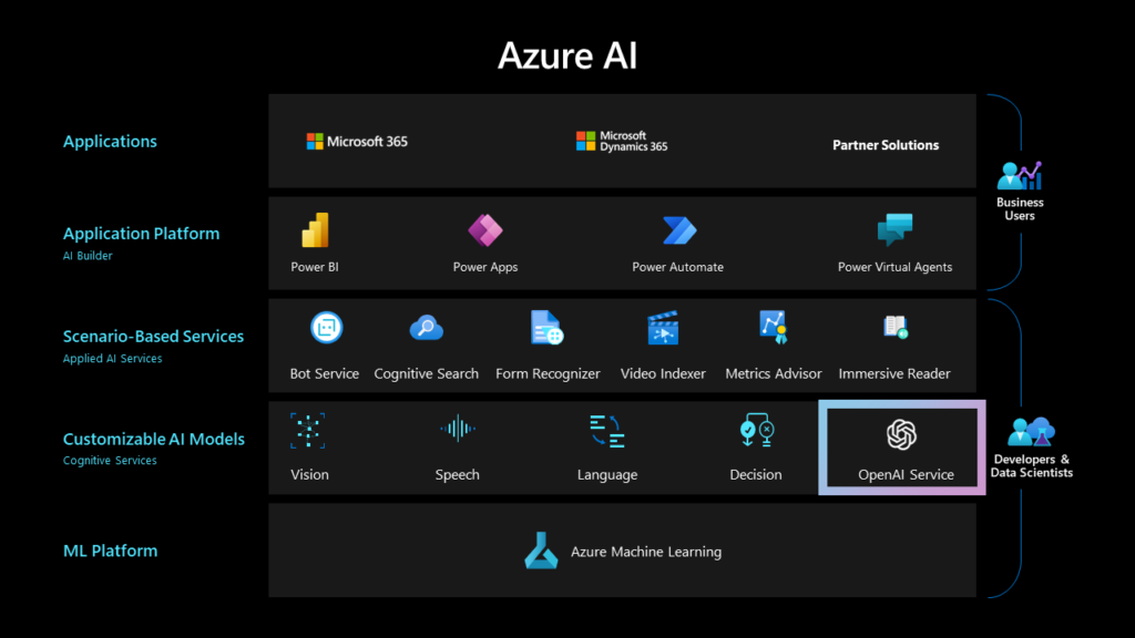


A slide presenting the Azure AI offerings, highlighting key features.

If ChatGPT is all-in-one shop, then Microsoft prepared whole commercial district


Ethics


Now, with figures such as Elon Musk and Bill Gates cautioning against AI and its growth the question of ethics in research and development appears. And while it is rather improbable that ChatGPT, being just a weighed statistical model becomes Roko’s Basilisk – the dangers of automation, unethical data sourcing and increased dependence on quick and easy answers generated by ChatGPT – remain.


So what steps are taken during development of new generation of AI models to ensure that it does more good than bad and won’t go Skynet on the general populace?


Ethical principles: Microsoft has established a set of ethical principles that guide the development and deployment of AI. These principles include fairness, reliability and safety, privacy and security, inclusiveness, transparency, and accountability.


Bias detection and mitigation: Microsoft uses a combination of algorithms and human reviewers to detect and mitigate bias in its AI services. For example, it has developed tools that can identify and correct biased language in chatbots like ChatGPT.


Data privacy and security: Microsoft has strict policies and procedures in place to protect the privacy and security of user data. It also provides users with tools and settings to control how their data is used.


Explainability and transparency: Microsoft aims to make its AI services more explicable and transparent to users. It has developed tools like the AI Explainability 360 toolkit, which allows developers to understand and explain the decisions made by AI models.


Partnerships and collaborations: Microsoft collaborates with governments, NGOs, and academic institutions to ensure that its AI services are used for the social good. For example, it partners with organizations like UNICEF and the World Bank to develop AI solutions that address social and environmental challenges.


Responsible AI initiative: Microsoft has launched a Responsible AI initiative to promote the development and deployment of AI that is ethical, transparent, and trustworthy. The initiative includes a set of tools and resources that developers can use to build responsible AI solutions.


But all of those did not prevent the chatbot from being implicated in a civil libel case filed by Victorian Mayor Brian Hood who claims the AI chatbot falsely describes him as someone who served time in prison as a result of a foreign bribery scandal. Additionally, there are some questions about the regulations about data privacy that may be breached by ChatGPT, which resulted in it being banned in Italy.


The watchdog organization being the bad referred to „the lack of a notice to users and to all those involved whose data is gathered by OpenAI” and said there appears to be „no legal basis underpinning the massive collection and processing of personal data in order to 'train’ the algorithms on which the platform relies”. It is also telling that the AI researcher apologized and committed to working diligently and rebuilding violated trust.


So, while artificial intelligence presents enormous opportunities, and both Microsoft and OpenAI try to conduct their research in an ethical way, it is important to stay informed and watchful about potential dangers and opportunities.


To end the section about Microsoft’s strategy and development of AI products, the most important part must be mentioned – pricing.


The answer for the questions about using GPT for business is simple – tokenization


The prices itself can and probably will change, as demand stabilizes, but the “pay-as-you-go” model is promising and allows for great flexibility as well as somehow predictable costs. Additionally, there are few AI models to choose from, either focusing on “reasoning” ability or cutting costs.


Summary


All in all, Microsoft’s AI strategy and partnership with OpenAI have the potential to significantly shape the future of AI technology and its applications across various industries. By democratizing AI, integrating AI capabilities into its products, and fostering strategic collaborations, Microsoft is poised to remain at the forefront of the AI revolution, driving innovation and enabling unprecedented advancements in the field. Most importantly for the company, they want users to depend on their productivity increasing services and providers of AI-based solutions to depend on their infrastructure and processing power.


This is a natural extension of Microsoft business strategy, but differently than Azure or Power BI – their hegemony in the AI-sphere is as of now nearly uncontested. Even Google seems to be unable to find the right answer, perhaps because their own AI, Bard, has a habit of providing the wrong ones. For us, mere mortals, all is left to do is keep abreast of developments, hope that ethics prevail during the research and be prepared for a world run with or by AI.


All content in this blog is created exclusively by technical experts specializing in Data ConsultingData InsightData Engineering, and Data Science. Our aim is purely educational, providing valuable insights without marketing intent.

bg

Artificial Intelligence Microsoft and OpenAI

How Microsoft acts to become the most important provider of AI backed services? Read and learn!

Read more arrow

Data Vault 3.0 – The summary


After the second part of the article series about Data Vault where we talked about data modelling and architecture, we return to you with quik look into naming conventions as well as the summary of the topic. It is great opportunity to learn something new, or just refresh your knowledge about Data Vault.


Naming convention


As we have already seen, the Data Vault is a multitude of tables with different structures and purposes. With hundreds of such objects in the warehouse, it is impossible to use them if we do not set the right naming rules.


Below is a sample set of prefixes for Data Vault objects:


Layer Data Vault object Name prefix
RDV Hub H_
RDV Satellite S_
RDV Multiactive satellite SM_
RDV Relational link L_
RDV Hierarchical link LH_
RDV Non-hierarchical link LT
BDV Hub BH_
BDV Satellite BS_
BDV Multiactive satellite BSM_
BDV Relational link BL_
BDV Hierarchical link BLH_
BDV Non-hierarchical link BLT
Other PIT PIT_
Other Bridge BR_
Other View V_<DV_object_prefix>


In addition to prefixes, it is worth standardizing the naming of related objects such as satellites around a common HUB and the naming of links. It is worth naming technical and business columns consistently. A dictionary of abbreviations and a dictionary of column prefixes and suffixes can be introduced.


Recap


If you’ve made it this far, you should already have a rough idea of what Data Vault is, how to create it, and what its advantages are. In my opinion, in order for the methodology to be used correctly it is also necessary to be aware of its disadvantages in order to prepare for their mitigation. For me, the fundamental disadvantage of Data Vault is the multiplicity of tables in the model and the difficulty in connecting them. Let’s say we want to write a cross-sectional query that retrieves data from three business hubs. Let’s say we need data from 2 satellites connected to each of these hubs (that’s already 9 tables). In addition, there are links between the hubs, and if there are satellites attached to the links, they also have to be included, which gives a total of (9+4) 13 tables that we have to involve.
 

This creates challenges in several areas:

  • Performance
  • Difficulty in writing SQL queries for the model
  • Difficulty in documenting the model


Of course, each of these points can be addressed, but it requires additional work that one should be aware of.


The fragmentation of tables is, on the one hand, a disadvantage that I mentioned above, but on the other hand, it also has its advantages. For data warehouses with multiple consumers, many sources, and many critical processes, fragmentation helps to minimize the impact of any errors in data feeding. For example, we read a small dictionary from a CSV file and based on it, calculate a column in the Data Vault satellite. When this file does not appear or appears with an error, we will not feed only that one satellite in the data warehouse.


The rest of the data warehouse will work correctly, and the processes based on it. In the case of choosing a different modeling approach, where broad tables are created, a problem with one small element can cause a problem with feeding one of the most important data warehouse tables, delaying most critical processes. Fragmentation also makes data storage more efficient – we store data immediately after it appears. There are no situations where we wait for data from, for example, five sources, which we then combine in ETL and store. It is clear that in such an approach, ETL can only start after all the input data has appeared, so the writing is delayed by this waiting time, unlike in Data Vault.


Fragmentation also helps in developing a data warehouse in many independent teams and releasing such changes. Data Vault is very „agile” and greater gradation of data and feeding processes means we have fewer dependencies between teams. It looks completely different when we have critical and broad tables in the model and many teams that modify them. In such cases, conflicts are not difficult, and the effort required for integration and regression testing is much greater.


How to effectively manage a Data Vault model? I don’t want to give advice on when to create a new satellite and under what rules, because in my opinion it must be tailored to the company and how the data warehouse is to be developed. However, I would like to draw attention to the elements that must be addressed in order not to fail during the development of a Data Vault model consisting of hundreds of tables.


First of all, the production process should be described, which establishes the rules for developing the data warehouse, from the moment the data requirements appear to the implementation stage and then maintenance. I will not go into details here because this is a topic for a separate article, but I will only emphasize the fact that the model must be properly documented, that the rules for development (adding additional tables to the model) should be defined, that object and column naming should be consistent, and that a framework should be created to automate the feeding of DV objects (calculating keys, hdif, partitioning, etc.). It is also best for such a fragmented model to refer to something at a more generalized level. In the company, a high-level Corporate Data Model should be created, which the fragmented model must be consistent with (we always model down: CDM -> Data Vault Model).


The Data Vault model is a business-oriented approach to data, not source systems. Business concepts are usually constant, while IT systems live and change much more often. If we want to have a consistent model that does not change with the exchange of the IT system underneath, then Data Vault is the right choice. However, is it recommended for every organization? Definitely not. If you want to integrate several dozen or hundreds of data sources in the company, and if the company does not have dozens or hundreds of critical processes, then Data Vault is unecessary. The overhead required for a proper solution preparation can also be significant. The larger planned data warehouse is, the more certain the Return On Investment (ROI). ROI increases when:

  • the number of source systems is large
  • source systems change frequently
  • the number of planned critical processes is significant
  • we plan to develop the model in many independent teams


So is Data Vault right for you? To answer your question you will need thorough understanding of your business needs and strategy, as well as knowledge about adventages and weaknesses od Data Vault. However, after reading our Data Vault series, you should be much better equipped to start answering the question.


This concludes the third and final part of our series of articles about Data Vault and its implementation. However, if you are curious about experts opinion and insights about data science, integration of data engineering solutions and synergizing technological and business strategy during data transformation – you are in luck!

Our experts create comperhensive and informative articles about the data analytic business. So tune in on our site and social media linked below to not miss valuable content.


And if you have additional questions about data – let’s talk about it!


All content in this blog is created exclusively by technical experts specializing in Data ConsultingData InsightData Engineering, and Data Science. Our aim is purely educational, providing valuable insights without marketing intent.

bg

Data Vault Part 3 - Summary

What is Data Vault? How to implement it in your organization and how to harness its power in your organization? Take a look and learn!

Read more arrow

Data Vault 2.0 – data model

After the first part of the article  series about Data Vault where we introduced the concept and the basicis of its architecture, we return to you with more in-depth look into data modeling. We will analyze concepts such as Business keys (BKEYs), hash keys (HKEYs), Hash diff (HDIF) and more!


Data Vault – technical columns


Business Key (BKEY)


In contrast to traditional data warehouses, Data Vault does not generate artificial keys on its own, nor does it use concepts such as sequences or key tables. Instead, it relies on a carefully selected attribute from the source system, known as the Business Key (BKEY). Ideally, the BKEY should not change over time and be the same across all source systems where the data is generated. While this may not always be possible, it greatly simplifies passive model integration. Furthermore, in the context of GDPR requirements, it is not advisable to choose business keys that contain sensitive data as it can be challenging to mask such data when exposing the data warehouse.


Examples of BKEYs may include the VAT invoice number, the accounting attachment number, or the account number. However, finding a suitable BKEY may not be an easy task. One best practice is to check how the business retrieves data from source systems and which values are used when entering data into the source system. Typically, these values, as they are known to the business, are good candidates for BKEYs. Often, the same data is processed in multiple source systems. For instance, in an organization with several systems for processing tax documents (invoices, receipts), natural document numbers (receipt/invoice numbers) may be used in some, while an artificial key (attachment number) may be used in others. In some cases, a sequential document number and an equivalent natural number are also used. In such situations, using an integration matrix can help identify the appropriate BKEY.


Table showcasing potential BKEY keys

Matrix showcasing potential BKEY keys


As we can see from the matrix, there are several potential BKEY keys, but only the document number appears in the majority of the sources from which we retrieve document data. If we use a BKEY key based on the document number, the data in the Data Vault model will naturally integrate. However, what will we get for data from „System 2„? For this data, we need to design an appropriate same-as link (a Data Vault object) that will connect the same data. More on this in the later part of the article.


It is important that the same BKEY keys from different source systems are loaded in the same way. Even if we want to format such a key, for example, by adding a constant prefix, we should do it in the same way for data from all sources.


Hash key (HKEY)


In the DV model, all joins are performed using a hash key. The hash key is the result of applying a hash function (such as MD5) to the BKEY value. The hash key is ideal for use as a distribution key for architectures with multiple data nodes and/or buckets. Through distribution, we can efficiently scale queries (insert and select) and limit data shuffling, as data with the same BKEY values are stored on the same node (having received the same HKEY).


Example BKEY and HKEY.Example BKEY and HKEY:


Hash diff (HDIF)


In Data Vault objects that store historical data (SCD2), HDIF represents the next versions of a record. HDIF is calculated by computing a hash value on all the meaningful columns in the table.


LoadTime


Date and hour of record loading.


DelFlag


Indication that a record has been deleted. It is important to note that in Data Vault 2.0 it is not recommended to use validity periods (valid from – valid to) to maintain historical records. As this requires costly update operations that are not efficient, especially for real-time data. In addition, for some Big Data technologies, update operations may not be available, which further complicates the implementation of validity periods. Instead, Data Vault recommends an insert-only architecture based on technical columns such as LoadTime and DelFlag to indicate when a record has been deleted.


Source


For Data Vault tables that receive data from multiple sources, the source column allows for additional partitioning (or sub-partitioning) to be established. Proper management of the physical structure of the table enables independent loading of data from multiple sources at the same time.

Different types of Data Vault objects have different sets of technical columns, which will be discussed further in the article.


Passive integration:


In classic warehouses, there are often so-called key tables in which keys assigned to business objects on a one-off basis are stored. Loading processes read the key table and, based on this, assign artificial keys in the warehouse. There are also sequences based on which keys are assigned, and sometimes a GUID is used.


All these solutions require additional logic to be implemented so that the value of the keys can be assigned consistently in the warehouse model. Often, these additional algorithms also limit the scalability of the warehouse resource. Passive integration is the opposite of this approach. Passive integration involves calculating a key on the fly during a table feed based only on the business key. With a deterministic transformation (hash function on BKEY), we can do this consistently in any dimension, e.g:


  • model dimension – the same BKEY in different warehouse objects will give us the same hkey so we can feed them independently and then combine them in any consistent way


  • time dimension – feeding the same BKEY at different points in time will give us the same result. Records powered up a year ago and today will get the same HKEY. Clearing the data and feeding it again will also have no effect on the calculated values (unlike, for example, in the case of sequences)


  • environment dimension – the same BKEY will have the same HKEY on different environments which facilitates testing and development.


The above is possible, but only if we choose the BKEY correctly, so the necessary effort should be made to make the choice optimal. We should consistently calculate it with the same algorithm for all HUB objects in the model. The exception can appear when we know that we have potential BKEYs in different formats in the source systems, but a simple transformation will make it consistent. It is important that this transformation is of the 'hard rule’ type.


For example:


In system 1 we have the key BKEY: „qwerty12345”


In system 2 we have the key BKEY: „QWERTY12345”


We know that business-wise they mean the same thing. In this case, we can apply a „hard rule” in the form of a LOWER or UPPER function to make the keys consistent.


Unfortunately, there are also situations where we have completely different BKEYs in different systems, for example:


In system 1 we have the key BKEY: „qwerty12345”


In system 2 we have the key BKEY: „7B9469F1-B181-400B-96F7-C0E8D3FB8EC0”


For such cases, we are forced to create so-called same-as links, which we will discuss later in this article.


Physical objects in Data Vault


Data Vault objects appear in the same form in both the RDV and BDV layers. The differences between them are only in the way the values in these objects are calculated (Hard rules and Soft rules). The objects of each layer should be distinguished at the level of naming convention and/or schema or database


RDV

  1. HUB
  2. LINK
  3. SATELLITE
    • Standard
    • Effectiveness
    • Multiactivity


BDV

  1. Business HUB
  2. Business LINK
  3. Business SATELLITE
    • Standard
    • Effectiveness
    • Multiactivity


HUB type objects


Hubs in the Data Vault warehouse are objects around which a grid of other related objects (satellites and links) is created. A Hub is a 'bag’ for business keys. A Hub cannot contain technical keys that the business does not understand, the keys must be unique. Examples of HUBs could be: customer, bill, document, employee, product, payment, etc.


We feed the Hubs with keys (BKEY) from the source systems, one BKEY can represent data from multiple source systems. We can use some rules to calculate BKEY but only those that meet the hard rules (usually UPPER, LOWER, TRIM). We never delete data from the HUB, if a record has disappeared from the source systems then its key should remain in the HUB. Even if the data is loaded into the hub in error, we do not need to delete unnecessary keys.


Example HUB structure, description of technical columns one chapter earlier.Example HUB structure, description of technical columns one chapter earlier.


Satellite type objects


It stores business attributes. We can have satellites with history (SCD2) or without history (SCD0/SCD1). We create a new satellite when we want to separate some group of attributes. We can do this for a number of reasons:


a) we want to store data of the same business importance (e.g. address data) in one place


b) we want to separate fast-changing attributes into a separate satellite. Fast-changing attributes are those that change frequently causing duplication of records in the satellite. Examples of such attributes could be e.g. interest rate, account balance, accrued interest, etc.


c) we want to segregate attributes with sensitive data for which we will apply restrictive permission policies or GDPR rules.


d) we want to add a new system to the warehouse and create a new satellite for it


e) others that for some reason will be optimal for us


Data Vault is very flexible in this respect. However, be sure to document the model well.


Diagram showing an example of a satellite with data recorded in SCD2 mode. Example of a satellite with data recorded in SCD2 mode:


Multiactive satellite – a specific type of a satellite where the key is not only BKEY but also a special multiactivity determinant (one of the substantive attributes). An example of such a satellite is a satellite storing address data where the multiactivity determinant is the type of address (correspondence, main, residential).


We have one BKEY (e.g. login in the application) and several addresses. We can successfully replace the multiactivity satellite with a regular one by adding a multiactivity determinant column to the hashkey calculation. My experience shows that it is better to limit the use of multiactivity satellites for reasons of model readability and reading efficiency.


 Diagram showing an example of a multiactivity satellite with data recorded in SCD2 modeExample of a multiactivity satellite with data recorded in SCD2 mode
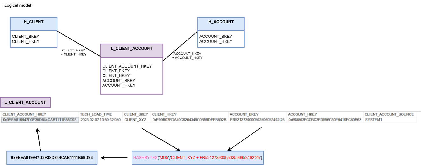
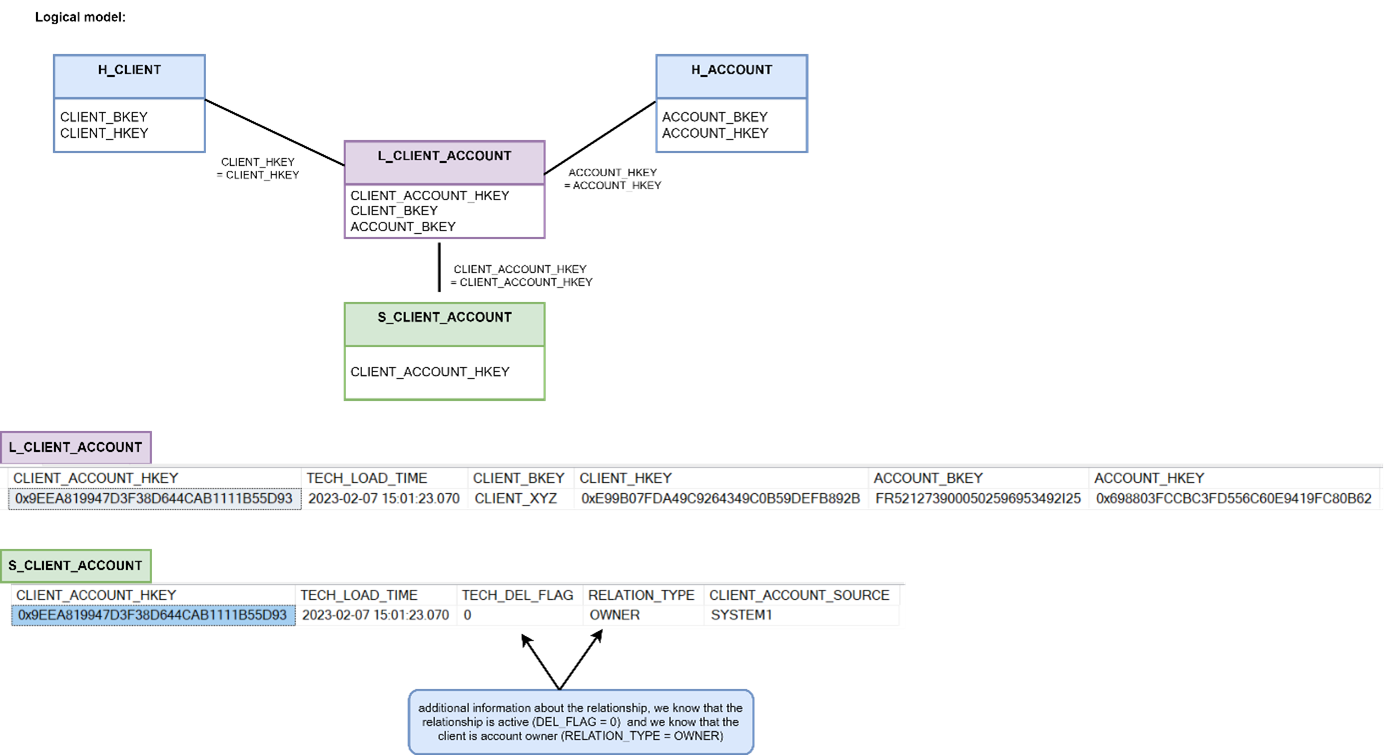


Link type objects


Link objects come in several versions:


Relational link – represents relationships between two or more objects which can be powered by complex business logic. Relationships must be unique – this is achieved by generating a unique hash for the relationship which is calculated from the hashes of the records it links. A link does not contain business columns (the exception is an nonhistorized link).

Diagram showing relationships between two or more objects which can be powered by complex business logic.


If we want to show history then we need to attach a satellite with a timeline to the link (effectivity satellite). The performance satellite can also contain additional business columns describing relationships.


Diagram showing the performance satellite containing additional business columns describing relationships.


Hierarchical link – used to model parent-child relationships (e.g. organisational structure) This type of link can of course also store history. To achieve that – just add an efficiency satellite to the link.


A diagram illustrating an example of an organizational structure in the Data Vault model, featuring a hierarchical link to represent relationships between entities and an efficiency satellite for tracking performance metricAn example of an organisational structure in the Data Vault model using a hierarchical link and an efficiency satellite:


Non-historicised link  (also known as transactional links) – a link that may contain business attributes within it, or may be associated with a satellite which has these attributes. The important thing is that it stores information about events that have occurred and will never be changed (like a classic fact table). Examples of such data are: system logs, invoice postings that can only be changed/withdrawn with another posting (storno accounting), etc.


A diagram showing an example of a non-historicized link in a Data Vault model.and example of a Non-historicised link


Link same as – allows you to tag different BKEY keys in the HUB table that essentially mean the same thing business-wise. I have mentioned this in previous chapters when describing the selection of the optimal BKEY. It is very important to note that this link only combines BKEY keys that business mean the same thing, we do not use the same as to register relationships other than mutually explicit relationships. We can use advanced algorithms to calculate often non-obvious links and record the results of the calculation in the link.


A diagram illustrating a "same as" link in a Data Vault model, showing the relationship between two hubs representing identical business entities, consolidating data from multiple sources.Examples of “same as” link


Links such as „same as” can be used in situations when we want to indicate often non-obvious business relationships, but also in very mundane situations. For example, when two systems have completely different business keys that represent the same thing, or when a key changes over time and we want to capture and record that change.


PIT facility – The Data Vault model is fragmented, as we have many subject satellites correlated to HUBs. Queries in the warehouse often involve several HUBs and satellites correlated with them. Selecting data from a specific point in time can be a challenge for the database. To improve read performance we use Point In Time (PIT) objects. A PIT table is something like a business index.


The important point is that we create PITs for specific business requirements. We define a set of source data (hubs, satellites), combine selected tables of hubs, links and satellites in such an arrangement as the business expects, e.g. for a selected moment in time (selected timeline or other business parameter). These are objects that we can reload and clean at any time, depending on the requirements of the recipient and the limitations of the hardware/system platform. The PIT is constructed from keys that refer to the hub and satellites so that we can retrieve data from these objects with a simple „inner join„.


A PIT facility can also refer to links instead of HUBs and satellites attached to a link.


BRIDGE object – works similarly to the PIT object with the difference being that it does not speed up access to data on a specific date but speeds up reading of a specific HKEY. Like PIT objects, BRIDGE objects are also created for the specific requirements of the data recipient. Bridge objects contain keys from multiple links and associated HUBs.


A diagram illustrating a RIDGE object in a Data Vault model.


The raw Data Vault model is not an easy model to use, it is difficult to navigate without documentation and therefore should not be made widely available to end users. The PIT as well as the Bridge objects help the end-user to read the DataVault data efficiently but it is important to remember that they are not a replacement for the Information Delivery (Data Mart) layers. They should be considered more as a bridge and/or optimisation object to produce higher layers. Of course, creating a PIT/Bridge object also costs money, so this optimisation method is used where there are many potential customers.


This concludes the second part of our series of articles about Data Vault and its implementation. Next week, you will be able to read about naming convention. Additionally, you will be able to find the summary of the information provided so far! To make sure you will not miss the next part of the series, be sure to follow us on our social media linked below. And if you have additional questions about data – let’s talk about it!


All content in this blog is created exclusively by technical experts specializing in Data ConsultingData InsightData Engineering, and Data Science. Our aim is purely educational, providing valuable insights without marketing intent.

bg

Data Vault Part 2 - Data modeling

What is Data Vault? How to implement it in your organization and how to harness its power in your organization? Take a look and learn!

Read more arrow

Introduction


Data Vault, compared to other modelling methods is relatively new. There are not many specialists with experience when it comes to data warehouses in this architecture. The lack of practical knowledge often results in solutions that only partially comply with the guidelines. This results in achieved results not fulfilling expectations and not supporting business strategy properly. Implementation and performance are especially problematic and require in-depth consideration.


But if you are curious about enormous potential of Data Vault as a Data Governance tool – you came to right place. Tomasz Dratwa, BitPeak Senior Data Engineer and Data Governance expert with several years of experience in implementing and developing Data Vaults decided to write down the most vital issues that need to be considered while building DV in your organization. Issues such as implementation of modelling from the architecture level to the physical fields in the warehouse. We are sure that they will help anyone who considers a warehouse in a Data Vault architecture.


The article is mostly for people who have some experience in dealing with databases and data warehouses before. It does not explain the basics of creating a data warehouse, modeling, foreign keys, or what SCD1 and SCD2 are. For those unfamiliar with the concepts, the article may be a challenging lecture. However, for those well-versed in dealing with databases and data warehouses, or just determined and able to access the google – this will most certainly be a very valuable lecture.


What is Data Vault?


Data Vault is a set of rules/methodologies that allow for the comprehensive delivery of a modern, scalable data warehouse. Importantly, these methodologies are universal. For example, they allow for modeling both financial data warehouses where data is loaded on a daily basis, and where backward data corrections are important, as well as warehouses collecting user behavioral data loaded in micro-batches. Data Vault precisely defines the types of objects in which data is physically stored, how to connect them, and how to use them. Thanks to these rules, we can create a high-performance (in terms of reading and writing) fully scalable (in terms of computing power, space, and surprisingly, also manufacturing!) data warehouse. Proper use of Data Vault enables us to fully leverage the scaling capabilities of Cloud, Big Data, Appliance, RDBMS environments (in terms of space and computing power). Additionally, the structure of the model and its flexibility allows for parallel development of the data warehouse model by multiple teams simultaneously (e.g., in the Agile Nexus model).


The two logical layers of the integrated Data Vault model are:


  • Raw Data Vault – raw data organized based on business keys (BKEY) and „hard rules” transformations (explained later in the article).


  • Business Data Vault – transformed and organized data based on business rules.


Both layers can physically exist in one database schema, and it’s important to manage the naming convention of objects appropriately. An issue which I will explain later. The Information Delivery layer (Data Marts) should be built on top of the above layers in a way that corresponds to the business requirements. It doesn’t have to be in the Data Vault format, so I won’t focus on Information Delivery design in this article.


Currently, Data Vault is most popular in Scandinavian countries and the United States, but I believe it is a very good alternative to Kimball and Immon and will quickly gain popularity worldwide.


Data Vault is „Business Centric” data model, which follows the business relationships rather than the systems and technical data structure in the sources. The data is grouped into areas, of which the central points are the so-called Hub objects (which will be discussed later). The technical and business timelines are completely separated. We can have multiple timelines because the time attributes in Data Vault are ordinary attributes of the data warehouse and do not have to be technical fields. On the other hand, Data Vault ensures data retention in the format in which the source system produced it, without loss or unnecessary transformations. It seems impossible to reconcile, yet it can be done.


Data Vault is a single source of facts, but the information an often be multi-faceted. Variants are necessary, because the same data is often interpreted differently by different recipients, and all these interpretations are correct. Facts are data as it came from the source; Such data can be interpreted in many ways, and with time, new recipients may appear for whom calculated values are incomplete. With time, the algorithms used for calculations may also degrade. Data Vault is fully flexible and prepared for such cases.


Data Vault is based on three basic types of objects/tables:


  • Hub: stores only business keys (e.g. document number).
  • Relational Link: contains relationships between business keys (e.g. connection between document number and customer).
  • Satellite: stores data and attributes for the business key from the Hub. A satellite can be connected to either a Hub or a Link.


 An example excerpt from a Data Vault model.

An example excerpt from a Data Vault model:


As you can see, the Data Vault model is not simple. Therefore, it is recommended to establish the appropriate rules for its development and documentation during the planning phase. It is also important to start modeling from a higher level. The best practice is to build a CDM (Corporate Data Model) in the company, which is a set of business entities and dependencies that function in the enterprise. The Data Vault model should refer to the high-level CDM in its detailed structure. Additionally, it is worth defining naming conventions for objects and columns. It is also necessary to document the model (e.g. in the Enterprise Architect tool).


Data Vault 2.0 – Architecture


In this article, we will focus only on the portion of the architecture highlighted on the diagram. To this end I will explain what the RDV and BDV layers are, how to model them logically and physically, and how to approach data modeling in relation to the entire organization. We will also discuss all types of Data Vault objects, good and bad practices for creating business keys, naming conventions, explain what passive integration is, and discuss hard rules and soft rules. I will try to cover all the key aspects of Data Vault, understanding of which enables the correct implementation of the data warehouse.


A high-level diagram of a data warehouse architecture based on the Data Vault model.
High-level diagram of a data warehouse architecture based on Data Vault.


Buisness hard and soft rules


A crucial aspect of a data warehouse is the storage and computation of facts and dimensions. To optimize this process, it’s very important to understand the differences between hard and soft rules transformations. Typically, the lower levels of any data warehouse store data in its least transformed state. This is due to practical considerations, as storing data in the form it was received in is crucial. Why? Because it allows us to use that data even after many years and calculate what we need at any given moment. On the other hand, some transformations are fully reversible and invariant over time, such as converting dates to the ISO format or converting decimal values from Decimal(14,2) to Decimal(18,4). These data transformations in Data Vault are called Hard Rules. Sometimes, we also consider irreversible transformations (for example trimming) as Hard Rules, but we must ensure that the data loss doesn’t have a business or technical impact. All other computations that involve column summation, data concatenation, dictionary-based calculations, or more complex algorithms fall under soft rule transformations. Data Vault clearly defines where we can apply specific transformations.


Raw Data Vault and Business Data Vault


In logical terms, the Data Vault model is divided into two layers:


Raw Data Vault (RDV) – Which contains raw data, with solely hard rules allowed for calculations. Despite this, the RDV model is fully business-oriented, with objects such as Hubs, Links, and Satellites arranged according to how the business understands the data. Technical data layouts, as found in the source system, are not allowed in this layer. This is known as the „Source System Data Vault (SSDV)”, which provides no benefits, such as passive model integration, which will be discussed later. This layer stores a longer history of data according to the needs of the data consumers. It is also a good practice to standardize the source system data types in this layer, for example, by having uniform date and currency formats.


Business Data Vault (BDV) – which allows for any type of data transformation (both hard and soft rules) and arranges the data in a business-oriented manner. The source of data for this layer is always the RDV layer. The fundamental rule of Data Vault is that the BDV layer can always be reconstructed based on the RDV layer. If all objects in the BDV layer are deleted, a well-constructed Data Vault model should allow for its re-population.


Both layers are accessible to users of the data warehouse and their objects can be easily combined. It is recommended to store tables from both the RDV and BDV layers in the same database (or schema) and differentiate them with an appropriate naming convention. 


This concludes the first part of our articles about Data Vault and its implementation. Next week, you will be able to read about data modelling. To make sure you will not miss the next part of the series, be sure to follow us on our social media linked below. And if you have additional questions about data – let’s talk about it!


All content in this blog is created exclusively by technical experts specializing in Data ConsultingData InsightData Engineering, and Data Science. Our aim is purely educational, providing valuable insights without marketing intent.


bg

Data Vault Part 1 - Introduction

What is Data Vault? How to implement it in your organization and how to harness its power in your organization? Take a look and learn!

Read more arrow

Introduction

As Artificial Intelligence develops, the need for more and more complex models of machine learning and more efficient methods to deploy them arises. The will to stay ahead of the competition and the interest in the best achievable process automation require implemented methods to get increasingly effective. However, building a good model is not an easy task. Apart from all the effort associated with the collection and preparation of data, there is also a matter of proper algorithm configuration.


This configuration involves inter alia selecting appropriate hyperparameters – parameters which the model is not able to learn on its own from the provided data. An example of a hyperparameter is a number of neurons in one of the hidden layers of the neural network. The proper selection of hyperparameters requires a lot of expert knowledge and many experiments because every problem is unique to some extent. The trial and error method is usually not the most efficient, unfortunately. Therefore some ways to optimise the selection of hyperparameters for machine learning algorithms automatically have been developed in recent years.


The easiest approach to complete this task is grid search or random search. Grid search is based on testing every possible combination of specified hyperparameter values. Random search selects random values a specified number of times, as its name suggests. Both return the configuration of hyperparameters that got the most favourable result in the chosen error metric. Although these methods prove to be effective, they are not very efficient. Tested hyperparameter sets are chosen arbitrarily, so a large number of iterations is required to achieve satisfying results. Grid search is particularly troublesome since the number of possible configurations increases exponentially with the search space extension.


Grid search, random search and similar processes are computationally expensive. Training a single machine learning model can take a lot of time, therefore the optimisation of hyperparameters requiring hundreds of repetitions often proves impossible. In business situations, one can rarely spend indefinite time trying hundreds of hyperparameter configurations in search for the best one. The use of cross-validation only escalates the problem. That is why it is so important to keep the number of required iterations to a minimum. Therefore, there is a need for an algorithm, which will explore only the most promising points. This is exactly how Bayesian optimisation works. Before further explanation of the process, it is good to learn the theoretical basis of this method.


Mathematics on cloudy days

Imagine a situation when you see clouds outside the window before you go to work in the morning. We can expect it to rain during any day. On the other hand, we know that in our city there are many cloudy mornings, and yet the rain is quite rare. How certain can we be that this day will be rainy?


Such problems are related to conditional probability. This concept determines the probability that a certain event A will occur, provided that the event B has already occurred, i.e. P(A|B). In case of our cloudy morning, it can go as P(Rain| Clouds), i.e. the probability of precipitation provided the sky was cloudy in the morning. The calculation of such value may turn out to be very simple thanks to Bayes’ theorem.


Helpful Bayes’ theorem


This theorem presents how to express conditional probability using the probability of occurrence of individual events. In addition to P(A) and P(B), we need to know the probability of B occurring if A has occurred. Formally, the theorem can be written as:


 A diagram of Bayes' theorem, showcasing the equation illustrating the relationship between conditional probabilities and the concept of updating beliefs based on new evidence.


This extremely simple equation is one of the foundations of mathematical statistics [1].


What does it mean? Having some knowledge of events A and B, we can determine the probability of A if we have just observed B. Coming back to the described problem, let’s assume that we had made some additional meteorological observations. It rains in our city only 6 times a month on average, while half of the days start cloudy. We also know that usually only 4 out of those 6 rainy days were foreshadowed by morning clouds. Therefore, we can calculate the probability of rain (P(Rain) = 6/30), cloudy morning (P(Clouds) = 1/2) and the probability that the rainy day began with clouds (P(Clouds|Rain) = 4/6). Basing on the formula from Bayes’ theorem we get:


A Bayes' theorem featuring the equation represent the probability of rain given cloudy weather, visually linking the theorem to real-world weather conditions.


The desired probability is 26.7%. This is a very simple example of using a priori knowledge (the right-hand part of the equation) to determine the probability of the occurrence of a particular phenomenon.


Let’s make a deal


An interesting application of this theorem is a problem inspired by the popular Let’s Make A Deal quiz show in the United States. Let’s imagine a situation in which a participant of the game chooses one of three doors. Two of them conceal no prize, while the third hides a big bounty. The player chooses a door blindly. The presenter opens one of the doors that conceal no prize. Only two concealed doors remain. The participant is then offered an option: to stay at their initial choice, or to take a risk and change the doors. What strategy should the participant follow to increase their chances of winning?


Contrary to the intuition, the probability of winning by choosing each of the remaining doors is not 50%. To find an explanation for this, perhaps surprising, statement, one can use Bayes’ theorem once again. Let’s assume that there were doors A, B and C to choose from. The player chose the first one. The presenter uncovered C, showing that it didn’t conceal any prize. Let’s mark this event as (Hc), while (Wb) should determine the situation in which the prize is behind the doors not selected by the player (in this case B). We look for the probability that the prize is behind B, provided that the presenter has revealed C:


A diagram of Bayes' theorem featuring the equation illustrating the probability of winning a game based on prior outcomes and new evidence, visually connecting statistical concepts to competitive scenarios.


The prize can be concealed behind any of the three doors, so (P(Wb) = 1/3). The presenter reveals one of the doors not selected by the player, therefore (P(Hc) = 1/2). Note also that if the prize is located behind B, the presenter has no choice in revealing the contents of the remaining doors – he must reveal C. Hence (P(Hc|Wb) = 1). Substituting into the formula:


Monty Hall paradox featuring the equation that calculates the probabilities of winning based on the decision to switch or stay, illustrating the counterintuitive results of the game show scenario.


Likewise, the chance of winning if the player stays at the initial choice is 1 to 3. So the strategy of changing doors doubles the chance of winning! The problem has been described in the literature dozens of times and it is known as the Monty Hall paradox from the name of the presenter of the original edition of the quiz show [2].


Bayesian optimisation


As it is not difficult to guess, the Bayesian algorithm is based on the Bayes’ theorem. It attempts to estimate the optimised function using previously evaluated values. In the case of machine learning models, the domain of this function is the hyperparameter space, while the set of values is a certain error metric. Translating that directly into Bayes’ theorem, we are looking for an answer to the question what will the f function value be in the point xₙ, if we know its value in the points: x₁, …, xₙ₋₁.


To visualize the mechanism, we will optimise a simple function of one variable. The algorithm consists of two auxiliary functions. They are constructed in such a way, that in relation to the objective function f they are much less computationally expensive and easy to optimise using simple methods.


The first is a surrogate function, with the task of determining potential f values in the candidate points. For this purpose, regression based on the Gaussian processes is often used. On the basis of the known points, the probable area in which the function can progress is determined. Figure 1 shows how the surrogate function has estimated the function f with one variable after three iterations of the algorithm. The black points present the previously estimated values of f, while the blue line determines the mean of the possible progressions. The shaded area is the confidence interval, which indicates how sure the assessment at each point is. The wider the confidence interval, the lower the certainty of how f progresses at a given point. Note that the further away we are from the points we have already known, the greater the uncertainty.


 A graphical representation of the progression of the surrogate function, illustrating its evolution over iterations, with curves depicting the function's value changes and optimization steps in a mathematical or algorithmic context. Figure 1: The progression of the surrogate function


The second necessary tool is the acquisition function. This function determines the point with the best potential, which will undergo an expensive evaluation. A popular choice, in an acquisition function, is the value of the expected improvement of f. This method takes into account both the estimated average and the uncertainty so that the algorithm is not afraid to „risk” searching for unknown areas. In this case, the greatest possible improvement can be expected at xₙ = -0.5, for which f will be calculated. The estimation of the surrogate function will be updated and the whole process will be repeated until a certain stop condition is reached. The progression of several such iterations is shown in Figure 3.


 A graphical representation of the progression of the surrogate function, illustrating its evolution over iterations, with red curves depicting the function's value changes and optimization steps in a mathematical or algorithmic context.Figure 2: The progression of the acquisition function
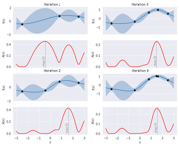


A diagram illustrating the progression of four iterations of the optimization algorithm, showing changes in function values and parameter adjustments across each iteration, highlighting the path toward convergence and improved solutions.
Figure 3: The progression of the four iterations of the optimisation algorithm


The actual progression of the optimised function with the optimum found is shown in Figure 4. The algorithm was able to find a global maximum of the function in just a few iterations, avoiding falling into the local optimum.
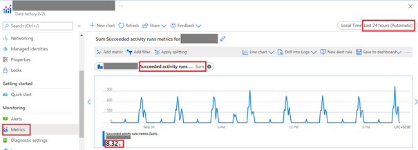
A graph displaying the actual progression of the optimized function, illustrating changes in function values over iterations, with marked improvements and convergence points that highlight the effectiveness of the optimization process.Figure 4: The actual progression of the optimised function


This is not a particularly demanding example, but it illustrates the mechanism of the Bayesian optimisation well. Its unquestionable advantage is a relatively small number of iterations required to achieve satisfactory results in comparison to other methods. In addition, this method works well in a situation where there are many local optima [3]. The disadvantage may be the relatively difficult implementation of the solution. However, dynamically developed open source libraries such as Spearmint [4], Hyperopt [5] or SMAC [6] are very helpful. Of course, the optimisation of hyperparameters is not the only application of the algorithm. It is successfully applied in such areas as recommendation systems, robotics and computer graphics [7].


References:

[1] „What Is Bayes’ Theorem? A Friendly Introduction”, Probabilistic World, February 22, 2016. https://www.probabilisticworld.com/what-is-bayes-theorem/ (provided July 15, 2020).

[2] J. Rosenhouse, „The Monty Hall problem. The remarkable story of math’s most contentious brain teaser”, January. 2009.

[3] E. Brochu, V. M. Cora, i N. de Freitas, „A Tutorial on Bayesian Optimization of Expensive Cost Functions, with Application to Active User Modeling and Hierarchical Reinforcement Learning”, arXiv:1012.2599 [cs], December. 2010

[4] https://github.com/HIPS/Spearmint

[5] https://github.com/hyperopt/hyperopt

[6] https://github.com/automl/SMAC3

[7] B. Shahriari, K. Swersky, Z. Wang, R. P. Adams, i N. de Freitas, „Taking the Human Out of the Loop: A Review of Bayesian Optimization”, Proc. IEEE, t. 104, nr 1, s. 148–175, January 2016, doi: 10.1109/JPROC.2015.2494218.


All content in this blog is created exclusively by technical experts specializing in Data ConsultingData InsightData Engineering, and Data Science. Our aim is purely educational, providing valuable insights without marketing intent.


bg

Smarter Artificial Intelligence with Bayesian Optimization

How to enhance Artifical Intelligence? Learn how to use Bayes’ theorem to optimize your machine learning models with us!

Read more arrow

Introduction


Data Factory is a powerful tool used in Data Engineers’ daily work in Azure cloud service. The code-free and user-friendly interface helps to clearly design data processes and improve Developer experience. It has many functionalities and features, which are constantly developed and enhanced by Microsoft.


The tool is mainly used to create, manage and monitor ETL (Extract-Transform-Load) pipelines which are the essence of the data engineering world. Therefore, I can confidently say that Data Factory has become the most integral tool in this field in Azure. But have you ever thought about the cost, that the service generates each time it is run? Have you ever done a deep dive into consumption run details, in order to investigate and explain the final price you have to pay each month for the tool?


Whether you have hundreds of long-running daily pipelines or use Data Factory for 10 minutes, once a week in your organization, it generates costs. Therefore, it is a good practice to know how to deal with it and create well-designed, cost-effective pipelines. In this article, you will find out how the small details can double your monthly invoice for Data Factory service. Azure is a pay-as-you-go service, which means that you pay only for what you actually used. However, the pricing details might overwhelm at first sight, and I hope the article will help you understand it more deeply. When you open official website (here or here) you can see that costs are divided into two parts: Data Pipeline and SQL Server Integration Services. In this article I will discuss only the Data Pipeline part, so let’s analyze it together.


Data Pipeline


First of all, it is important to realize that you are not only charged for executing pipelines, but the cost for Data Pipeline is calculated based on the following factors:

  1. Pipeline orchestration and execution
  2. Data flow execution and debugging
  3. Number of Data Factory operations (e.g. pipeline monitoring)


Pipeline orchestration


You are charged for data pipeline orchestration (activity run and activity execution) by integration runtime hours. Azure offers three different integration runtimes which provide the computing resources to execute the activities in pipelines. The below table presents the cost for each integration runtime.


Type Azure Integration Runtime Price Azure Managed VNET Integration Runtime Price Self-Hosted Integration Runtime Price
Orchestration 1$ per 1 000 runs 1$ per 1 000 runs 1.5$ per 1 000 runs
*the presented prices are for West Europe region in March 2022, source.


Orchestration refers to activity runs, trigger executions and debug runs. If you run 1000 activities using Azure Integration Runtime you are charged $1. The price seems to be low, but if you have a process that runs a lot of activities in loops many times a day, you could be surprised how much it could cost at the end of the month.


If you want to study existing pipelines in Data Factory, I recommend you to check the value in Data Factory/Monitoring/Metrics section by displaying charts Succeeded activity runs and Failed activity runs. The sum of these values is a total number of activity runs. The below picture presents how you can check the statistics for Data Factory instance for last 24 hours.


A screenshot of the Azure Data Factory dashboard, showcasing various data integration and transformation tools


As you can see in the above example, the pipelines are executed every 3 hours and the total number succeeded activity runs is 8320. How much does it cost? Let’s calculate:


Daily price: 8320/1000 * $1 = $8.32


Monthly price: 8320/1000 * $1 * 30 days = $249.6


Pipeline executions


Every pipeline execution generates cost. Pipeline activity is defined as an activity which is executed on integration runtime. The below table presents the pricing of execution Pipeline Activity and External Pipeline Activity. As demonstrated in the below table, the price is calculated based on the time of execution and the type of integration runtime.


Type Azure Integration Runtime Price Azure Managed VNET Integration Runtime Price Self-Hosted Integration Runtime Price
Pipeline Activity $0.005/hour $1/hour $0.10/hour
​External Pipeline Activity $0.00025/hour $1/hour $0.0001/hour
*the presented prices are for West Europe region in March 2022, source.

Depending on the type of activity that is executed in Data Factory, the price is different, as illustrated in Pipeline Activity and External Pipeline Activity sections in the table above. Pipeline Activities use computing configured and deployed by Data Factory, but External Pipeline Activities use computing configured and deployed externally to Data Factory. In order to show which activity belongs where, I prepared the below table.

Pipeline Activities External Pipeline Activities
Append Variable, Copy Data, Data Flow, Delete, Execute Pipeline, Execute SSIS Package, Filter, For Each, Get Metadata, If Condition, Lookup, Set Variable, Switch, Until, Validation, Wait, Web Hook Web Activity, Stored Procedure, HD Insight Streaming, HD Insight Spark, HD Insight Pig, HD Insight MapReduce, HD Insight Hive, U-SQL (Data Lake Analytics), Databricks Python, Databricks Jar, Databricks Notebook, Custom (Azure Batch), Azure ML, Execute Pipeline, Azure ML Batch Execution, Azure ML Update Resource, Azure Function, Azure Data Explorer Command
*source


Rounding up


While executing pipelines, you need you know that execution time for all activities is prorated by minutes and rounded up. Therefore, if the accurate execution time for your pipeline run is 20 seconds, you will be charged for 1 minute. You can notice that in the activity output details in the billingReference section. The below pictures present an example of executing Copy Data activity.


Output of data within 20 second depicted as text


The section billingReference in output details of execution of the activity holds information like meterType, duration, unit. The pipeline was executed on self-hosted integration runtime and lasted 1/60 min = 0.016666666666666666 hour, although the time of execution was 20 seconds.


Inactive pipelines


It was really surprising for me, that Azure charges for each inactive pipeline which has no associated trigger or zero runs within one month. The fee for it is $0.80 per month for every pipeline, so it is crucial to delete unused pipelines from Data Factory especially when you deal with hundreds of pipelines. If you have 100 unused pipelines in your project, the monthly fee is $80 and the yearly cost is $960.


Copy Data Activity


Copy Data window


Copy Data Activity is one of the options in Data Factory. You can use it to move the data from one place to another. It is important to know that in Settings you can change the default Auto value to 2. By doing so, you can decrease the data integration unit to a minimum, if you copy small tables. In general, the value of units can be in the range of 2-256 and Microsoft has recently implemented a new feature for Auto option. When you choose Auto, it means that Data Factory dynamically applies the optimal DIU setting based on your source-sink pair and data pattern.


The below table presents the cost of consumption of one DIU per hour for different types of integration runtime.


Type ​Azure Integration Runtime Price Azure Managed VNET Integration Runtime Price Self-Hosted Integration Runtime Price
Copy Data Activity $0.25/DIU-hour $0.25/DIU-hour $0.10/hour
*The presented prices are for West Europe region in March 2022, source.


Let’s estimate cost of a pipeline that has only Copy Data Activity.


Example:


If Copy Data Activity lasts 48 seconds, the copy duration time is rounded up to 1 minute, so the cost is equal to:


1 minute * 4 DIUs * $0.25 = 0.0167 hours * 4DIUs * $0.25 = $0.0167


As you can see the price $0.0167 seems to be low, but let’s consider it more deeply. If you execute the pipeline for 100 tables every day, the monthly cost is equal to:


$0.0167 * 100 tables *30 days = $50.1


If you execute the pipeline for 100 tables every single hour, the monthly cost is equal to:


$0.0167 * 100 tables * 30 days * 24 hours = $1,202.4


The most crucial part of creating the pipeline solution is to keep in mind that even if you handle small tables, but do it very often, it could dramatically increase the total cost of the execution. If it is feasible, I recommend preparing the data upfront and using one large file instead. You can just code a simple Python script.


Bandwidth


The next factor that could be relevant in regard to pricing is Bandwidth. If you want to transfer the data between Azure data centers or move in or out the data of Azure data centers you can be additionally charged. Generally, moving the data within the same region and inbound data transfer is free, but the situation could be different in other cases. The price depends on the region, internet Egress and differs for Intra-continental or Inter-continental data transfer.


For example, if you transfer 1000 GB data between regions within Europe, the price is $20, but in South America it is $160. When it is necessary to move 1000 GB from Europe to other continents the price is $50, but from Asia to other continents it’s $80. Therefore, think twice before you decide where to locate your data and how often you will have to transfer it. As you notice, there are many factors contributing to the bandwidth price. You can find the whole price list in Azure documentation.


Data Flow


A visual representation of the Azure Data Factory.


Data Flow is a powerful tool in ETL process in Data Factory. You can not only copy the data from one place to another but also perform many transformations, as well as partitioning. Data Flows are executed as activities that use scale-out Apache Spark clusters. The minimum cluster size to run a Data Flow is 8 vCores. You are charged for cluster execution and debugging time per vCore-hour. The below table presents Data Flow cost by cluster type.

Type Price
General Purpose $0.268 per vCore-hour
Memory Optimized $0.345 per vCore-hour
*the presented prices are for West Europe region in March 2022, source.


It is recommended to create your own Azure Integration Runtimes with a defined region, Compute Type, Core Counts and Time To Live feature. What is really interesting, is that you can dynamically adjust the Core Count and Compute Type properties by sizing the incoming source dataset data. You can do it simply by using activities such as Lookup and Get Metadata. It could be a useful solution when you cope with different dataset sizes of your data.


To sum up, in terms of Data Flows in general you are charged only for cluster execution and debugging time per vCore-hour, so it is significant to configure these parameters optimally. If you want to use one basic cluster (general purpose) for one hour and use a minimum number of Core Count, the total price of execution is equal to:


$0.268 * 8 vCores * 1 hour = $2,144


The monthly price is equal to:

$0.268 * 8 vCores * 30 days * 1hour = $64.32


There are four bottlenecks that depend on total execution time of Data Flow:

  1. Cluster start-up time
  2. Reading from source
  3. Transformation time
  4. Writing to sink

I want to focus on the first factor: cluster start-up time. It is a time period that is needed to spin up an Apache Spark cluster, which takes approximately 3-5 minutes. By default, every data flow spins up a new Spark cluster, based on the Azure Integration Runtime configuration (cluster size etc.). Therefore, if you execute 10 Data Flows in a loop each time, a new cluster is spun up, ultimately it can last 30-50 minutes just for start-up clusters.


In order to decrease cluster start-up time, you can enable Time To Live option. The feature keeps a cluster alive for a certain period of time after its execution completes. So, in our example each Data Flow will reuse the existing cluster – it starts only once, and it takes 3-5 minutes instead of 30-50 minutes. Let’s assume that the cluster start-up lasts 4 minutes.

Scenario 1 – Estimated time of executing 10 Data Flows without Time To Live Scenario 2 – Estimated time of executing 10 Data Flows with Time To Live
Cluster start-up time 40 min 4 min (+ 10 min Time to Live)
Reading from source 10 min 10 min
Transformation time 10 min 10 min
Writing to sink 10 min 10 min


The table above presents two scenarios of execution 10 Data Flows in one pipeline, but the second option has Time To Live feature that lasts 10 minutes.


Cost of executing the pipeline in scenario 1:

70 mins/60 * $0.268 * 8 vCores = $2.5


Cost of executing the pipeline in scenario 2:

44mins/60 * $0.268 * 8 vCores = $1.57


It easy to see that the price in scenario 1 is much higher than in scenario 2.

The most crucial part of using Time to Live option is the way of executing the pipelines. It is highly recommended to use Time To Live only when pipelines contain multiple sequential Data Flows. Only one job can run on a single cluster at a time. When one Data Flow finishes, the second one starts. If you execute Data Flows in a parallel way, then only one Data Flow will use the live cluster and others will spin up their own clusters.


Moreover, each of them will generate extra cost from Time To Live feature, because clusters will wait unused for a certain period of time when they finish. In consequence, the cost could be higher than without Time To Live feature. In addition, before implementing the solution make sure if Quick Re-use option is turned on in integration runtime configuration. It allows to reuse a live cluster for many Data Flows.


Data Factory Operations


The next actions that generate cost are the „read”, „write” and „monitoring” options. The below table presents the pricing.

Type Price
Read/Write $0.50 per 50 000 modified/referenced entities
Monitoring $0.25 per 50 000 run records retrieved
the presented prices are for West Europe region in March 2022, source.

Read/write operations for Azure Data Factory entities include „create„, „read„, „update„, and „delete„. Entities include datasets, linked services, pipelines, integration runtime, and triggers. Monitoring operations include get and list for pipeline, activity, trigger, and debug runs. As you can see, every action in the data pipeline generates cost, but this factor is the least painful one when it comes to pricing, because 50 000 is really a huge number.


Monitor


I would like to present you one feature that could be helpful in finding bottlenecks in your existing solution in Data Factory. First of all, every executed pipeline is logged in Monitor section in Data Factory tool. Logs contain a data of every step of the ETL process, including pipeline run consumption details, but there they are stored for only 45 days in Monitor. Nevertheless, it is feasible to calculate an estimated price of Pipeline orchestration and Pipeline execution.


I found PowerShell code on Microsoft community website that generates aggregated data of pipelines run consumption within one resource group for defined time range. I strongly believe that the code can be useful for costs estimation of your existing pipelines. It is worth mentioning that this method has some limitations and for example it doesn’t contain information about consumption of Time To Live in Data Flows. In the picture below you can see this information in the red box.


Pipeline run consumpiotns and posible data thats is aviable to harvest


I hope you found this article helpful in furthering your understanding of pricing details and the features that could be significant in your solutions. Microsoft is still improving Data Factory and while preparing this paper I needed to change two paragraphs due to the changes in Azure documentation. For example, from January 2022, you will no longer need to manually specify Quick Re-use in Data Flows when you create an integration runtime and that is great information. I found a funny quote that could describe Azure pricing in general: You don’t pay for Azure services; you only pay for things you forget to turn off – or in this case – “turn on”.


All content in this blog is created exclusively by technical experts specializing in Data ConsultingData InsightData Engineering, and Data Science. Our aim is purely educational, providing valuable insights without marketing intent.

bg

The pricing explanation of Azure Data Factory

See how to optimize the costs of using Azure Data Factory!

Read more arrow

Digital Fashion — Clothes that aren’t there

Sitting in a cozy café in your favorite t-shirt, with one click you change into a shirt and put on a jacket. You can start a conference with your future client. Such perspective is becoming more and more real, and closer than ever, due to concept of Digital Fashion.


Digital clothes being worn on a meetng online

Pic. 1. Source


With the development of new technologies, especially 3D graphics (rendering, 3D models and fabric physics), the term is becoming increasingly popular. And what is Digital Fashion really? It is simply digital clothing – a virtual representation of clothing created using 3D software and then „superimposed” on a virtual human model.


Exploring digital fashion: 3D graphics and virtual clothing


Gif. 1. The Fabricant


Digital Fashion seems to be the next step in the development of the powerful e-commerce and fashion markets. Online stores started with descriptions and photos; now 360° product animations have become the norm, and digitally created models’ faces and bodies are increasingly being used for promotional graphics. The time for virtual fitting rooms and maybe even our own virtual wardrobes is coming. Actually, this (r)evolution has already taken its first steps. Let us just look at AR app projects of brands such as Nike (2019) or the collaboration of Italian fashion house Gucci with Snapchat (2020).


Virtual shoe fitting with AR technology: the evolution of digital fashion

Gif. 2. Application for virtual shoe fitting. Source


Where did the need for this type of solution come from? The main, but not the only, factors giving rise to this type of application are:


On-line work and social relations – more and more events are moving or taking place simultaneously in the virtual world. The same applies to professions and even social gatherings. Remote working „via webcam” is no longer the domain of the IT industry, but increasingly appears in the entire sectors of the economy.


Environmental consciousness — digital clothes and accessories do not require farmland or animal husbandry for fabric and leather, as well as 93 billion cubic meters of water to produce textiles, laundry detergents, or global distribution routes. Designed once anywhere in the world, they can be globally available in no time.


The rapid increase in the popularity of items that do not exist in the real world – NFTs (non-fungible tokens) and people adopting digital alter egos.


The new generations are natives of technology. They largely communicate, and thus express themselves, in the virtual world. A perfect example of this trend is the success of fashion house Balenciaga’s campaign done in cooperation with the game Fortnite. Digital-to-Physical Partnerships will become more and more common.


Above, I have only outlined the emerging niche of Digital Fashion. It is also worth mentioning Polish achievements in this field – those interested may refer to the VOGUE article on the Nueno digital clothing brand and the article on homodigital.pl. Personally, I am extremely curious what virtual reality will bring to the e-commerce and fashion market in the coming years.


The rise of digital fashion: virtual clothing by Stephy Fung

Pic.2. Digital Clothes made by STEPHY FUNG.


VR/DF Application — Big Picture

The rapid development of the Digital Fashion niche observed in recent years gives us huge, still largely undiscovered opportunities for the development of new products and services in this area. From designers specializing only in Digital Fashion, through professionals selecting textures for virtual fabrics, to programmers responsible for the unique physics of clothes. Personally, my favorite option would probably be to turn off gravity – you are sitting safely in a chair, and the shirt you’re wearing is acting like you’re in outer space. So naturally, space is created for apps that showcase emerging products and for marketplaces where customers will be able to view and purchase them.


For the purpose of this article, we will take on the challenge of creating just such a solution – an AR app connected to a digital clothing marketplace. The application will give the user the to create their own virtual styling, and clothing brands, as well as related brands, to officially sell their products and NFT.


Basic application principles

In theory, the operation is very simple – the application collects data about the user’s posture from the camera image, then processes it in real time using a library for human pose estimation (technology: OpenCV + Python). The collected data is actually just points in 3D space. They are transferred to the 3D engine, in which a virtual model of the User is created. The 3D model of the character itself is invisible, but interacts with visible clothes and/or accessories (technology: Blender 3D + Python). Ultimately, the user sees himself with the digital clothing superimposed.


Diagram of the components of the application responsible for the virtual scene.
Pic. 3. Diagram of the components of the application responsible for the virtual scene.


At this point, it is worth clarifying two terms:


POSE ESTIMATION — pose estimation is a computer vision technique that predicts movements and tracks the location of a person. We can also think of pose estimation as the problem of determining the position and orientation of a camera relative to an object. This is usually done by identifying, locating and tracking a number of key points on a person, such as the wrist, elbow or knee.


RIGGING(skeletal animation) means equipping a 3D model of a human, animal or other character with jointed limbs and virtual bones.These form a skeleton inside the model, which makes it much easier and more efficient for the animator to maneuver – movements of the bones affect the movement of the 3D model.


The exchange of information between the program making the pose estimation and the skeleton inside the human model is the basis of the created application. Data packets about the position of characteristic points on the body, which are x, y, z parameters in space, will be connected with the same points in rigging of the 3D model of the figure.


Overlaying points from pose estimation on the joints of a 3D human modelPic. 4. Overlaying points from pose estimation on the joints of a 3D human model.


General guidelines for business objectives

The proposed solution does not go in the direction of a virtual avatar (i.e. it does not position itself as a replacement for a person’s image). We are interested in the environment around the person, in the surroundings – clothes, accessories, interiors, etc. – what is around is already a product. Following the proverb „closer to the body than the shirt”, the closest and always fashionable product are clothes – hence we will strongly focus on this segment of the market.


The question arises – what if the user wants to change their eye color? From there it’s close to swapping your hand for that of the Terminator after the fight in the final scene. I identify such needs as very interesting (e.g. in Messenger filters), but infantile. I would describe the proposed solution as a place of man + product, rather than man + visual modification of man. This is intended to imply an image of greater maturity, professionalism and brand awareness. In practice, it is meant to be a place where existing brands can sell products right away. The product focus is also meant to clearly differentiate this solution from the filters familiar from TikTok/Instagram, or animated emoticons on iOS.


Clothing in Metaverse

Just how fresh and hot the topic of digital clothing, and the entire emerging market associated with it is, is indicated by the huge interest generated by the Connect 2021 conference, during which the CEO of Facebook, or, for some, META, presented the Metaverse (’meta’- beyond, and 'universum’- world). This is the concept of a new internet combining the 'internet of things’ with the 'internet of people’. Mark Zuckerberg explained in an interview with The Verge that the Metaverse is „an embodied internet where instead of just viewing content – you are in it”. The author of the term itself is Neal Stephenson, who used it nearly thirty years ago in his cyberpunk book Snow Crash. In it, he describes the story of people living simultaneously in two realities – real and virtual.


The question is not „will it happen?” but rather „when and how it will happen?” As augmented, and virtual reality technologies become increasingly present in our lives, the world that now surrounds us on a daily basis will migrate into the Metaverse. Offices, pubs, gyms, flats are all now our mundane lives and will also be present in digital life. At the center, however, will always be people and their experiences. But what would interactions with others be like without the right attire? A „burning” t-shirt of your favorite band at a virtual concert; a waterfall dress during a New Year’s Eve meta-ball, or a golden shirt at a business meeting summarizing a successful project – although it sounds like science-fiction, this series of articles is an attempt to respond to such needs.


Digital clothing in Metaverse showing mark Zuckerberg in digital and reality

Gif.3. Digital clothing in Metaverse


Conclusion

The evolution of the e-commerce market towards Digital Fashion has already begun. This is possible thanks to the dynamic development of technologies such as Pose Estimation, 3D graphics, and hundreds of other smaller, but very important, innovations appearing every day. In this article, we’ve given an overview of what digital clothing is and the opportunities it presents – for software developers on the one hand, and designers and graphic designers on the other.


In the future articles we will focus on technical issues related to the created application and market. Those interested can count on a large dose of code in Python associated with Pose Estimation and Blender 3D. There will also be plenty of news related to Digital Fashion and Metaverse.


All content in this blog is created exclusively by technical experts specializing in Data ConsultingData InsightData Engineering, and Data Science. Our aim is purely educational, providing valuable insights without marketing intent.

bg

Clothes that aren't there. AR and Python in the Digital Fashion.

Sitting in a cozy café in your favorite t-shirt, with one click you change into a shirt and put on a jacket.

Read more arrow

Introduction

AWS Glue is an arsenal of possibilities for data engineers to create ETL processes with Amazon resources. It supports a setup of calculating units where jobs can be in the form of Python or Spark scripts made from scratch or using AWS Glue Studio with an interactive visual designer. The designer has a simple interface and comes up with helpful set of ready to use transformations. Still, it also presents some limitation and problems.

The Limitations

The visual designer automatically generates a script for every added transformation. This script can be modified, however, any change to it will block the possibility for further visual development as user code cannot be translated into visual transformations.


Currently there are 15 available transformations, like Select Fields, Join, or Filter. Those basic operations cover up most of typical data operations, yet there is always a need for more complex calculations. In those situations, SQL and Custom transformations come to the rescue. First one extends the job’s capabilities only to SQL functions. Second one allows to create a new transformation with user made Python function that can only accept one parameter and always need to return DynamicFrameCollection.


If there is a need to extend a job with additional parameters they need to be added in the job’s configuration, yet they are also needed to be added manually to the script. If a developer builds the job with visual templates, it makes them impossible to do the development further in the visual designer, as a proper visual operation to add jobs’ parameters into script is not implemented.


The Problems 

Some transformations, like SelectFields, do not handle empty datasets in a proper manner. If empty dataset needs to be processed, those transformations will return an empty object without headers. This in turn will lead to an error in the next step, if any processing is applied on the indicated columns.


There are several problems with the web interface itself, i.e., a significant amount of used visual transformation leads to a complete slowdown of the designer, or if someone wants to change the data type for only one column in ApplyMapping with selection menu, this sometimes causes unexpected changes in all other columns.


Data preview is a great addition to AWS Glue Studio as it allows to observe how parts of data are processed through every transformation. However, if there is any error in a job, it prints a general error message and restarts itself to print the same message on and on. This does not allow to really validate the error, which sometimes forces you to stop viewing the Data preview and run the job in standard mode.


All content in this blog is created exclusively by technical experts specializing in Data ConsultingData InsightData Engineering, and Data Science. Our aim is purely educational, providing valuable insights without marketing intent.

bg

AWS Glue– Tips for Beginners Part II. Limitation of AWS Glue Studio

AWS Glue is an arsenal of possibilities for data engineers to create ETL processes with Amazon resources.

Read more arrow

Introduction to Case Study

AWS Glue is, amongst other AWS services, a great choice for a Big Data project. Alone or even with other services, like AWS Step Function and AWS EventBridge, it may help create a fully operational system for data analysis and reporting. The service provides ETL functionalities, facilitates integration with different data sources and allows a flexible approach to development.


In the following paragraphs I present a review of AWS Glue features and its functionalities based on a real example of integration with external databases and loading data form there to S3 buckets. Whole purpose of this exercise is to present technical side of the service using a practical case and building a simple solution step by step.

The Connection

In the reviewed case, the data source is a PostgreSQL database which is an external resource from AWS. It stores few tabular datasets that are supposed to be moved to Amazon S3. Someone could create a connection to scan this database directly In a form of a script, but here we can use AWS Glue Connections. It allows to create a static connection to databases which stores connection’s definition, the chosen user and its password. It delivers a possibility to connect external databases, Amazon RDS, Amazon Redshift, MongoDB and others.

Crawlers

Based on the established connection in AWS Glue, it is possible to scan databases to know what tables are available there. Developers can use AWS Glue Crawlers which may analyse whole databases model for a chosen database schema to create an internal representation of tables. A Crawler can be run manually or based on a schedule to scan one or more data sources. A successful scan of Crawler creates metadata in Data Catalog for Databases and Tables.

Databases and Tables

Databases in AWS Glue serve a purpose of containers for inferred Tables. Tables are just metadata and they reference actual data in an external source, i.e., their data are not saved in Amazon storage. In a situation where inferred Tables are created with Crawler scanning internal Amazon resources, those Tables would also act only as references. This means that deleting Tables in AWS Glue would only lead to deletion of metadata in Data Catalog, but not to deletion of physical resources on external databases or S3. What developers must also remember is that Tables from external resources are not available for ad-hoc queries using Amazon Athena, even though scanned Databases exists in Amazon Athena.

The Jobs

AWS Glue lets developers create Spark or simple Python jobs, where jobs’ settings can be modified to select type of workers, number of workers, timeouts, concurrency, additional libraries, job parameters and so on. Developers may create a job by writing and passing scripts using Amazon platform or using recent feature in AWS Glue Studio to create jobs with a visual designer.


AWS Glue job extracting, filtering, and storing data in S3 with generated script

Picture presents a Glue Studio job in a visual form (left) and its representation in code (right).


Continuing with the case study, in the above picture there is a visually created job that would import data from PostgreSQL databases into S3 bucket. In this simple example, there are only three operations used (left side of the picture): Data source, Transform and Data target. Those operations and additional other built-in transformations simplify the process of creating Glue jobs. First operation directly creates a data frame from an external table by simply indicating Database and Table created in the previous steps. Then, by “filter” transformation, only specific data are saved into S3 bucket with the last operation.


All those three steps can be done manually just by the means of passing parameters in the visual designer. Moreover, visual transformations will generate a ready to run script (right side of the picture). This script can be modified, but that irreversibly switches off a possibility of further modification using the visual designer. This limitation only allows creation of simplest jobs or a start-up of bigger jobs.


The above steps show the features of AWS Glue. Some of them could be omitted, if one would like to create his/her own way of connecting to a different data source using credentials stored in AWS Secrets Manager instead of creating Connection in AWS Glue. Additionally, there are a couple more useful functions of AWS Glue that were omitted in this article, like Workflow, or Triggers. Apart from the nice sides of AWS Glue, there are some disadvantages that need to be taken into consideration. Those will be mentioned in next article about AWS Glue.


All content in this blog is created exclusively by technical experts specializing in Data ConsultingData InsightData Engineering, and Data Science. Our aim is purely educational, providing valuable insights without marketing intent.

bg

AWS Glue – Tips for Beginners. Part I – Review of the Service

AWS Glue is, amongst other AWS services, a great choice for a Big Data project.

Read more arrow
Load more
vector